Wave Equation

John S Butler john.s.butler@tudublin.ie Course Notes Github

Overview

This notebook will implement the Forward Euler in time and Centered in space method to appoximate the solution of the wave equation.

The Differential Equation

Condsider the one-dimensional hyperbolic Wave Equation:

(812)\[\begin{equation} \frac{\partial u}{\partial t} +a\frac{\partial u}{\partial x}=0,\end{equation}\]

where \(a=1\), with the initial conditions

(813)\[\begin{equation} u(x,0)=1-\cos(x), \ \ 0 \leq x \leq 2\pi. \end{equation}\]

with wrap around boundary conditions.

# LIBRARY
# vector manipulation
import numpy as np
# math functions
import math 

# THIS IS FOR PLOTTING
%matplotlib inline
import matplotlib.pyplot as plt # side-stepping mpl backend
import warnings
warnings.filterwarnings("ignore")

Discete Grid

The region \(\Omega\) is discretised into a uniform mesh \(\Omega_h\). In the space \(x\) direction into \(N\) steps giving a stepsize of

(814)\[\begin{equation} \Delta_x=\frac{2\pi-0}{N},\end{equation}\]

resulting in

(815)\[\begin{equation}x[j]=0+j\Delta_x, \ \ \ j=0,1,...,N,\end{equation}\]

and into \(N_t\) steps in the time \(t\) direction giving a stepsize of

(816)\[\begin{equation} \Delta_t=\frac{1-0}{N_t}\end{equation}\]

resulting in

(817)\[\begin{equation}t[n]=0+n\Delta_t, \ \ \ n=0,...,K.\end{equation}\]

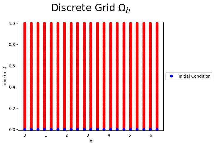
The Figure below shows the discrete grid points for \(N=10\) and \(Nt=100\), the known boundary conditions (green), initial conditions (blue) and the unknown values (red) of the Heat Equation.

N=20
Nt=100
h=2*np.pi/N
k=1/Nt
time_steps=100
time=np.arange(0,(time_steps+.5)*k,k)
x=np.arange(0,2*np.pi+h/2,h)

X, Y = np.meshgrid(x, time)

fig = plt.figure()
plt.plot(X,Y,'ro');
plt.plot(x,0*x,'bo',label='Initial Condition');
plt.xlim((-h,2*np.pi+h))
plt.ylim((-k,max(time)+k))
plt.xlabel('x')
plt.ylabel('time (ms)')
plt.legend(loc='center left', bbox_to_anchor=(1, 0.5))
plt.title(r'Discrete Grid $\Omega_h$ ',fontsize=24,y=1.08)
plt.show();

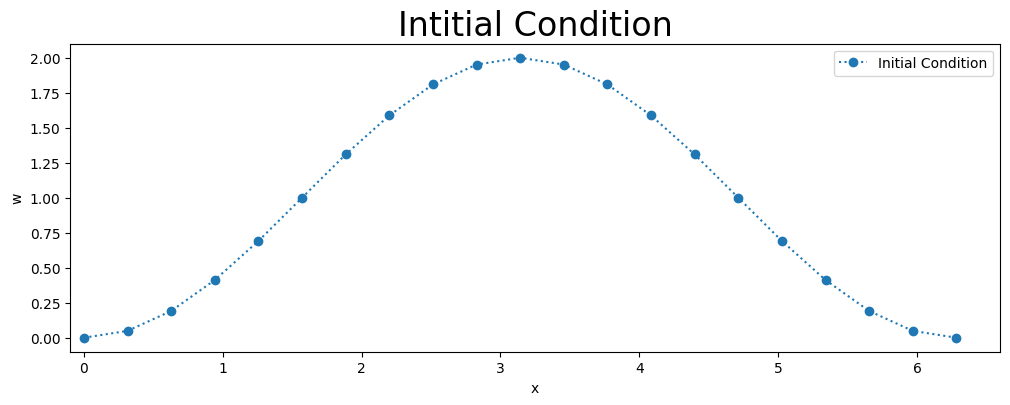
Initial Conditions

The discrete initial conditions is,

(818)\[\begin{equation} w[0,j]=1-\cos(x[j]), \ \ 0 \leq x[j] \leq \pi, \end{equation}\]

The figure below plots values of \(w[j,0]\) for the inital (blue) conditions for \(t[0]=0.\)

w=np.zeros((time_steps+1,N+1))
b=np.zeros(N-1)
# Initial Condition
for j in range (0,N+1):
    w[0,j]=1-np.cos(x[j])
    

fig = plt.figure(figsize=(12,4))
plt.plot(x,w[0,:],'o:',label='Initial Condition')
plt.xlim([-0.1,max(x)+h])
plt.title('Intitial Condition',fontsize=24)
plt.xlabel('x')
plt.ylabel('w')
plt.legend(loc='best')
plt.show()

Boundary Conditions

To account for the wrap-around boundary conditions

(819)\[\begin{equation}w_{-1,n}=w_{N,n},\end{equation}\]

and

(820)\[\begin{equation}w_{N+1,n}=w_{0,n}.\end{equation}\]

xpos = np.zeros(N+1)
xneg = np.zeros(N+1)

for j in range(0,N+1):
   xpos[j] = j+1
   xneg[j] = j-1

xpos[N] = 0
xneg[0] = N

The Explicit Forward Time Centered Space Difference Equation

The explicit Forward Time Centered Space difference equation of the Wave Equation is,

(821)\[\begin{equation} \frac{w^{n+1}_{j}-w^{n}_{j}}{\Delta_t}+\big(\frac{w^n_{j+1}-w^n_{j-1}}{2\Delta_x}\big)=0. \end{equation}\]

Rearranging the equation we get,

(822)\[\begin{equation} w_{j}^{n+1}=w^{n}_{j}-\lambda a(w_{j+1}^{n}-w_{j-1}^{n}), \end{equation}\]

for \(j=0,...10\) where \(\lambda=\frac{\Delta_t}{\Delta_x}\).

This gives the formula for the unknown term \(w^{n+1}_{j}\) at the \((j,n+1)\) mesh points in terms of \(x[j]\) along the nth time row.

lamba=k/h
for n in range(0,time_steps):
    for j in range (0,N+1):
         w[n+1,j]=w[n,j]-lamba/2*(w[n,int(xpos[j])]-w[n,int(xneg[j])])
       
        

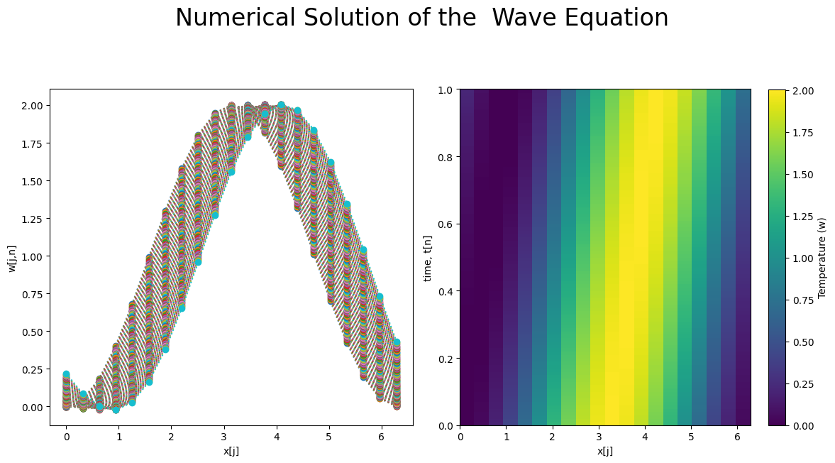
Results

fig = plt.figure(figsize=(12,6))

plt.subplot(121)
for n in range (1,time_steps+1):
    plt.plot(x,w[n,:],'o:')
plt.xlabel('x[j]')
plt.ylabel('w[j,n]')

plt.subplot(122)
X, T = np.meshgrid(x, time)
z_min, z_max = np.abs(w).min(), np.abs(w).max()


plt.pcolormesh( X,T, w, vmin=z_min, vmax=z_max)

#plt.xticks(np.arange(len(x[0:N:2])), x[0:N:2])
#plt.yticks(np.arange(len(time)), time)
plt.xlabel('x[j]')
plt.ylabel('time, t[n]')
clb=plt.colorbar()
clb.set_label('Temperature (w)')
#plt.colorbar()
plt.suptitle('Numerical Solution of the  Wave Equation',fontsize=24,y=1.08)
fig.tight_layout()
plt.show()