Finite Difference Method

John S Butler john.s.butler@tudublin.ie

Course Notes
Github

Overview

This notebook illustrates the finite different method for a linear Boundary Value Problem. The video below walks through the code.

from IPython.display import HTML
HTML('<iframe width="560" height="315" src="https://www.youtube.com/embed/DMtnJ7vrb8s" frameborder="0" allow="accelerometer; autoplay; clipboard-write; encrypted-media; gyroscope; picture-in-picture" allowfullscreen></iframe>')

/Users/johnbutler/opt/anaconda3/lib/python3.8/site-packages/IPython/core/display.py:724: UserWarning: Consider using IPython.display.IFrame instead
  warnings.warn("Consider using IPython.display.IFrame instead")

Introduction

To numerically approximate a linear Boundary Value Problem

(502)$$y^{{}^{″}}=f(x,y,y^{{}^{\prime }}),a<x<b,$$

with the boundary conditions

(503)$$y(a)=\alpha ,$$

(504)$$y(b)=\beta ,$$

is dicretised to a system of difference equations. the first derivative can be approximated by the difference operators:

(505)$$D^{+}{U}_i=\frac{U_{i+1}-U_i}{h_{i+1}}\text{ Forward,}$$

(506)$$D^{-}{U}_i=\frac{U_i-U_{i-1}}{h_i}\text{ Backward,}$$

or

(507)$$D^0{U}_i=\frac{U_{i+1}-U_{i-1}}{x_{i+1}-x_{i-1}}=\frac{U_{i+1}-U_{i-1}}{2h}\text{ Centered.}$$

The second derivative can be approximated by:

(508)$${\delta }_x^2{U}_i=\frac{2}{x_{i+1}-x_{i-1}}(\frac{U_{i+1}-U_i}{x_{i+1}-x_i}-\frac{U_i-U_{i-1}}{x_i-x_{i-1}})=\frac{U_{i+1}-2U_2+U_{i-1}}{h^2}\text{ Centered in }x\text{ direction}.$$

Example Boundary Value Problem

To illustrate the method we will apply the finite difference method to the this boundary value problem

(509)$$\frac{d^{2}y}{d{x}^2}=4y,$$

with the boundary conditions

(510)$$y(0)=1.1752,y(1)=10.0179.$$

import numpy as np
import math
import matplotlib.pyplot as plt
import warnings
warnings.filterwarnings("ignore")

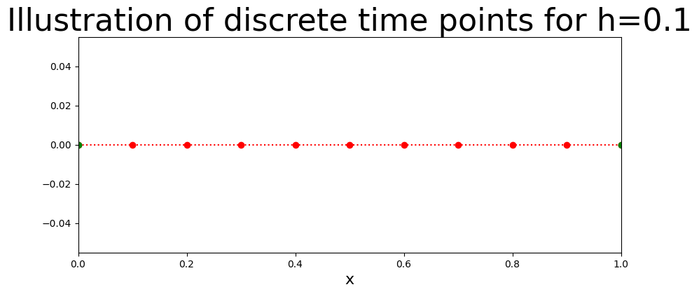
Discrete Axis

The stepsize is defined as

(511)$$h=\frac{b-a}{N}$$

here it is

(512)$$h=\frac{1-0}{10}$$

giving

(513)$$x_i=0+0.1i$$

for $i=0,1,...10.$

## BVP
N=10
h=1/N
x=np.linspace(0,1,N+1)
fig = plt.figure(figsize=(10,4))
plt.plot(x,0*x,'o:',color='red')
plt.plot(x[0],0,'o:',color='green')
plt.plot(x[10],0,'o:',color='green')


plt.xlim((0,1))
plt.xlabel('x',fontsize=16)
plt.title('Illustration of discrete time points for h=%s'%(h),fontsize=32)
plt.show()

The Difference Equation

To convert the boundary problem into a difference equation we use 1st and 2nd order difference operators. The general difference equation is

(514)$$\frac{1}{h^2}(y_{i-1}-2y_i+y_{i+1})=4y_{i}i=1,..,N-1.$$

Rearranging the equation we have the system of N-1 equations

(515)$$i=1:\frac{1}{{0.1}^2}{y}_0-(\frac{2}{{0.1}^2}+4)y_1+\frac{1}{{0.1}^2}{y}_2=0$$

(516)$$i=2:\frac{1}{{0.1}^2}{y}_1-(\frac{2}{{0.1}^2}+4)y_2+\frac{1}{{0.1}^2}{y}_3=0$$

(517)$$...$$

(518)$$i=8:\frac{1}{{0.1}^2}{y}_7-(\frac{2}{{0.1}^2}+4)y_8+\frac{1}{{0.1}^2}{y}_9=0$$

(519)$$i=9:\frac{1}{{0.1}^2}{y}_8-(\frac{2}{{0.1}^2}+4)y_9+\frac{1}{{0.1}^2}{y}_{10}=0$$

where the green terms are the known boundary conditions.

Rearranging the equation we have the system of 9 equations

(520)$$i=1:-(\frac{2}{{0.1}^2}+4)y_1+\frac{1}{{0.1}^2}{y}_2=-\frac{1}{{0.1}^2}{y}_0$$

(521)$$i=2:\frac{1}{{0.1}^2}{y}_1-(\frac{2}{{0.1}^2}+4)y_2+\frac{1}{{0.1}^2}{y}_3=0$$

(522)$$...$$

(523)$$i=8:\frac{1}{{0.1}^2}{y}_7-(\frac{2}{{0.1}^2}+4)y_8+\frac{1}{{0.1}^2}{y}_9=0$$

(524)$$i=9:\frac{1}{{0.1}^2}{y}_8-(\frac{2}{{0.1}^2}+4)y_9=-\frac{1}{{0.1}^2}{y}_{10}$$

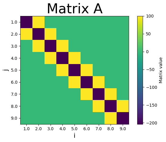
where the green terms are the known boundary conditions. This is system can be put into matrix form

(525)$$A\mathbf{y}=\mathbf{b}$$

Where A is a $9\times 9$ matrix of the form

(526)$$A=\left(\begin{array}{ccccccccc}-204& 100& 0& 0& 0& 0& 0& 0& 0\\ 100& -204& 100& 0& 0& 0& 0& 0& 0\\ 0& 100& -204& 100& 0& 0& 0& 0& 0\\ .& .& .& .& .& .& .& .& .\\ .& .& .& .& .& .& .& .& .\\ 0& 0& 0& 0& 0& 0& 100& -204& 100\\ 0& 0& 0& 0& 0& 0& 0& 100& -204\end{array}\right)$$

which can be represented graphically as:

A=np.zeros((N-1,N-1))
# Diagonal
for i in range (0,N-1):
    A[i,i]=-(2/(h*h)+4)

for i in range (0,N-2):           
    A[i+1,i]=1/(h*h)
    A[i,i+1]=1/(h*h)
    
plt.imshow(A)
plt.xlabel('i',fontsize=16)
plt.ylabel('j',fontsize=16)
plt.yticks(np.arange(N-1), np.arange(1,N-0.9,1))
plt.xticks(np.arange(N-1), np.arange(1,N-0.9,1))
clb=plt.colorbar()
clb.set_label('Matrix value')
plt.title('Matrix A',fontsize=32)
plt.tight_layout()
plt.subplots_adjust()
plt.show()

$\mathbf{y}$ is the unknown vector which is contains the numerical approximations of the $y$. $$ \color{red}{\mathbf{y}}=\color{red}{ \left(\begin{array}{c} y_1\ y_2\ y_3\ .\ .\ y_8\ y_9 \end{array}\right).} \end{equation}

y=np.zeros((N+1))
# Boundary Condition
y[0]=1.1752
y[N]=10.0179

and the known right hand side is a known $9\times 1$ vector with the boundary conditions

(527)$$\mathbf{b}=\left(\begin{array}{c}-117.52\\ 0\\ 0\\ .\\ .\\ 0\\ -1001.79\end{array}\right)$$

b=np.zeros(N-1)

# Boundary Condition
b[0]=-y[0]/(h*h)
b[N-2]=-y[N]/(h*h)

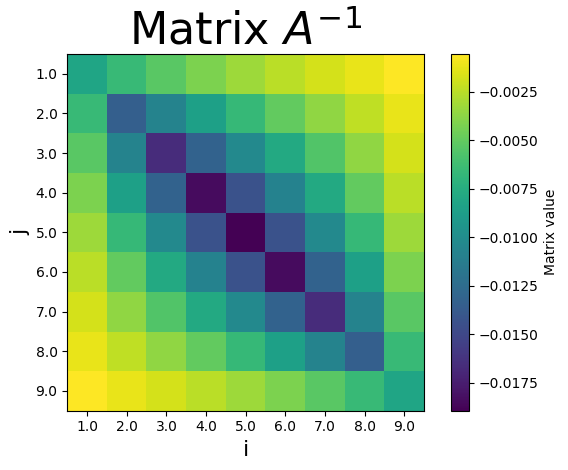
Solving the system

To solve invert the matrix $A$ such that

(528)$$A^{-1}Ay=A^{-1}b$$

(529)$$y=A^{-1}b$$

The plot below shows the graphical representation of $A^{-1}$.

invA=np.linalg.inv(A)

plt.imshow(invA)
plt.xlabel('i',fontsize=16)
plt.ylabel('j',fontsize=16)
plt.yticks(np.arange(N-1), np.arange(1,N-0.9,1))
plt.xticks(np.arange(N-1), np.arange(1,N-0.9,1))
clb=plt.colorbar()
clb.set_label('Matrix value')
plt.title(r'Matrix $A^{-1}$',fontsize=32)
plt.tight_layout()
plt.subplots_adjust()
plt.show()


y[1:N]=np.dot(invA,b)

Result

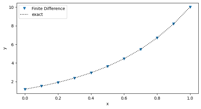
The plot below shows the approximate solution of the Boundary Value Problem (blue v) and the exact solution (black dashed line).

fig = plt.figure(figsize=(8,4))

plt.plot(x,y,'v',label='Finite Difference')
plt.plot(x,np.sinh(2*x+1),'k:',label='exact')
plt.xlabel('x')
plt.ylabel('y')
plt.legend(loc='best')
plt.show()