The Implicit Backward Time Centered Space (BTCS) Difference Equation for the Heat Equation

John S Butler john.s.butler@tudublin.ie Course Notes Github

Overview

This notebook will implement the implicit Backward Time Centered Space (FTCS) Difference method for the Heat Equation.

The Heat Equation

The Heat Equation is the first order in time (\(t\)) and second order in space (\(x\)) Partial Differential Equation:

(563)\[\begin{equation} \frac{\partial u}{\partial t} = \frac{\partial^2 u}{\partial x^2},\end{equation}\]

the equation describes heat transfer on a domain

(564)\[\begin{equation} \Omega = \{ t \geq, 0\leq x \leq 1\}. \end{equation}\]

with an initial condition at time \(t=0\) for all \(x\) and boundary condition on the left (\(x=0\)) and right side (\(x=1\)).

Backward Time Centered Space (BTCS) Difference method

This notebook will illustrate the Backward Time Centered Space (BTCS) Difference method for the Heat Equation with the initial conditions

(565)\[\begin{equation} u(x,0)=2x, \ \ 0 \leq x \leq \frac{1}{2}, \end{equation}\]

(566)\[\begin{equation}u(x,0)=2(1-x), \ \ \frac{1}{2} \leq x \leq 1, \end{equation}\]

and boundary condition

(567)\[\begin{equation} u(0,t)=0, u(1,t)=0. \end{equation}\]

# LIBRARY
# vector manipulation
import numpy as np
# math functions
import math 

# THIS IS FOR PLOTTING
%matplotlib inline
import matplotlib.pyplot as plt # side-stepping mpl backend
import warnings
warnings.filterwarnings("ignore")

Discete Grid

The region \(\Omega\) is discretised into a uniform mesh \(\Omega_h\). In the space \(x\) direction into \(N\) steps giving a stepsize of

(568)\[\begin{equation} h=\frac{1-0}{N},\end{equation}\]

resulting in

(569)\[\begin{equation}x[i]=0+ih, \ \ \ i=0,1,...,N,\end{equation}\]

and into \(N_t\) steps in the time \(t\) direction giving a stepsize of

(570)\[\begin{equation}k=\frac{1-0}{N_t}\end{equation}\]

resulting in

(571)\[\begin{equation}t[i]=0+ik, \ \ \ k=0,...,K.\end{equation}\]

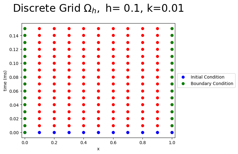
The Figure below shows the discrete grid points for \(N=10\) and \(Nt=100\), the known boundary conditions (green), initial conditions (blue) and the unknown values (red) of the Heat Equation.

N=10
Nt=100
h=1/N
k=1/Nt
r=k/(h*h)
time_steps=15
time=np.arange(0,(time_steps+.5)*k,k)
x=np.arange(0,1.0001,h)
X, Y = np.meshgrid(x, time)
fig = plt.figure()
plt.plot(X,Y,'ro');
plt.plot(x,0*x,'bo',label='Initial Condition');
plt.plot(np.ones(time_steps+1),time,'go',label='Boundary Condition');
plt.plot(x,0*x,'bo');
plt.plot(0*time,time,'go');
plt.xlim((-0.02,1.02))
plt.xlabel('x')
plt.ylabel('time (ms)')
plt.legend(loc='center left', bbox_to_anchor=(1, 0.5))
plt.title(r'Discrete Grid $\Omega_h,$ h= %s, k=%s'%(h,k),fontsize=24,y=1.08)
plt.show();

Discrete Initial and Boundary Conditions

The discrete initial conditions are

(572)\[\begin{equation} w[i,0]=2x[i], \ \ 0 \leq x[i] \leq \frac{1}{2} \end{equation}\]

(573)\[\begin{equation} w[i,0]=2(1-x[i]), \ \ \frac{1}{2} \leq x[i] \leq 1 \end{equation}\]

and the discete boundary conditions are

(574)\[\begin{equation} w[0,j]=0, w[10,j]=0,\end{equation}\]

where \(w[i,j]\) is the numerical approximation of \(U(x[i],t[j])\).

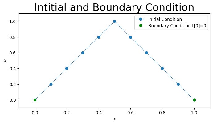
The Figure below plots values of \(w[i,0]\) for the inital (blue) and boundary (red) conditions for \(t[0]=0.\)

w=np.zeros((N+1,time_steps+1))
b=np.zeros(N-1)
# Initial Condition
for i in range (1,N):
    w[i,0]=2*x[i]
    if x[i]>0.5:
        w[i,0]=2*(1-x[i])
    

# Boundary Condition
for k in range (0,time_steps):
    w[0,k]=0
    w[N,k]=0

fig = plt.figure(figsize=(8,4))
plt.plot(x,w[:,0],'o:',label='Initial Condition')
plt.plot(x[[0,N]],w[[0,N],0],'go',label='Boundary Condition t[0]=0')
#plt.plot(x[N],w[N,0],'go')
plt.xlim([-0.1,1.1])
plt.ylim([-0.1,1.1])
plt.title('Intitial and Boundary Condition',fontsize=24)
plt.xlabel('x')
plt.ylabel('w')
plt.legend(loc='best')
plt.show()

The Implicit Backward Time Centered Space (BTCS) Difference Equation

The implicit Backward Time Centered Space (BTCS) difference equation of the Heat Equation is derived by discretising

(575)\[\begin{equation} \frac{\partial u_{ij+1}}{\partial t} = \frac{\partial^2 u_{ij+1}}{\partial x^2},\end{equation}\]

around \((x_i,t_{j+1})\) giving the difference equation

(576)\[\begin{equation} \frac{w_{ij+1}-w_{ij}}{k}=\frac{w_{i+1j+1}-2w_{ij+1}+w_{i-1j+1}}{h^2} \end{equation}\]

Rearranging the equation we get

(577)\[\begin{equation} -rw_{i-1j+1}+(1+2r)w_{ij+1}-rw_{i+1j+1}=w_{ij} \end{equation}\]

for \(i=1,...9\) where \(r=\frac{k}{h^2}\).

This gives the formula for the unknown term \(w_{ij+1}\) at the \((ij+1)\) mesh points in terms of \(x[i]\) along the jth time row.

Hence we can calculate the unknown pivotal values of \(w\) along the first row of \(j=1\) in terms of the known boundary conditions.

This can be written in matrix form

(578)\[\begin{equation} A\mathbf{w}_{j+1}=\mathbf{w}_{j} +\mathbf{b}_{j+1} \end{equation}\]

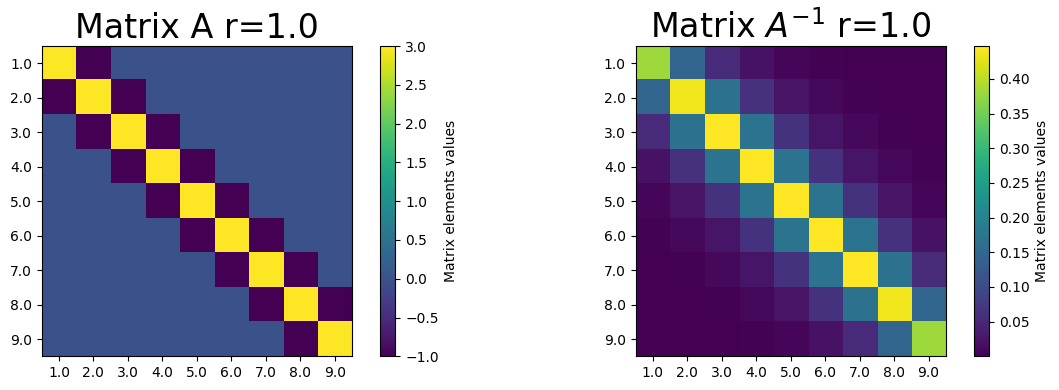
for which \(A\) is a \(9\times9\) matrix:

(579)\[\begin{equation} \left(\begin{array}{cccc cccc} 1+2r&-r& 0&0&0 &0&0&0\\ -r&1+2r&-r&0&0&0 &0&0&0\\ 0&-r&1+2r &-r&0&0& 0&0&0\\ 0&0&-r&1+2r &-r&0&0& 0&0\\ 0&0&0&-r&1+2r &-r&0&0& 0\\ 0&0&0&0&-r&1+2r &-r&0&0\\ 0&0&0&0&0&-r&1+2r &-r&0\\ 0&0&0&0&0&0&-r&1+2r&-r\\ 0&0&0&0&0&0&0&-r&1+2r\\ \end{array}\right) \left(\begin{array}{c} w_{1j+1}\\ w_{2j+1}\\ w_{3j+1}\\ w_{4j+1}\\ w_{5j+1}\\ w_{6j+1}\\ w_{7j+1}\\ w_{8j+1}\\ w_{9j+1}\\ \end{array}\right)= \left(\begin{array}{c} w_{1j}\\ w_{2j}\\ w_{3j}\\ w_{4j}\\ w_{5j}\\ w_{6j}\\ w_{7j}\\ w_{8j}\\ w_{9j}\\ \end{array}\right)+ \left(\begin{array}{c} rw_{0j+1}\\ 0\\ 0\\ 0\\ 0\\ 0\\ 0\\ 0\\ rw_{10j+1}\\ \end{array}\right). \end{equation}\]

It is assumed that the boundary values \(w_{0j+1}\) and \(w_{10j+1}\) are known for \(j=1,2,...\), and \(w_{i0}\) for \(i=0,...,10\) is the initial condition. The Figure below shows the values of the \(9\times 9\) matrix in colour plot form for \(r=\frac{k}{h^2}\).

A=np.zeros((N-1,N-1))
for i in range (0,N-1):
    A[i,i]=1+2*r

for i in range (0,N-2):           
    A[i+1,i]=-r
    A[i,i+1]=-r
    
Ainv=np.linalg.inv(A)   
fig = plt.figure(figsize=(12,4));
plt.subplot(121)
plt.imshow(A,interpolation='none');
plt.xticks(np.arange(N-1), np.arange(1,N-0.9,1));
plt.yticks(np.arange(N-1), np.arange(1,N-0.9,1));
clb=plt.colorbar();
clb.set_label('Matrix elements values');
#clb.set_clim((-1,1));
plt.title('Matrix A r=%s'%(np.round(r,3)),fontsize=24)

plt.subplot(122)
plt.imshow(Ainv,interpolation='none');
plt.xticks(np.arange(N-1), np.arange(1,N-0.9,1));
plt.yticks(np.arange(N-1), np.arange(1,N-0.9,1));
clb=plt.colorbar();
clb.set_label('Matrix elements values');
#clb.set_clim((-1,1));
plt.title(r'Matrix $A^{-1}$ r=%s'%(np.round(r,3)),fontsize=24)

fig.tight_layout()
plt.show();

Results

To numerically approximate the solution at \(t[1]\) the matrix equation becomes

(580)\[\begin{equation} \mathbf{w}_{1}=A^{-1}(\mathbf{w}_{0} +\mathbf{b}_{1}) \end{equation}\]

where all the right hand side is known. To approximate solution at time \(t[2]\) we use the matrix equation

(581)\[\begin{equation} \mathbf{w}_{2}=A^{-1}(\mathbf{w}_{1} +\mathbf{b}_{2}). \end{equation}\]

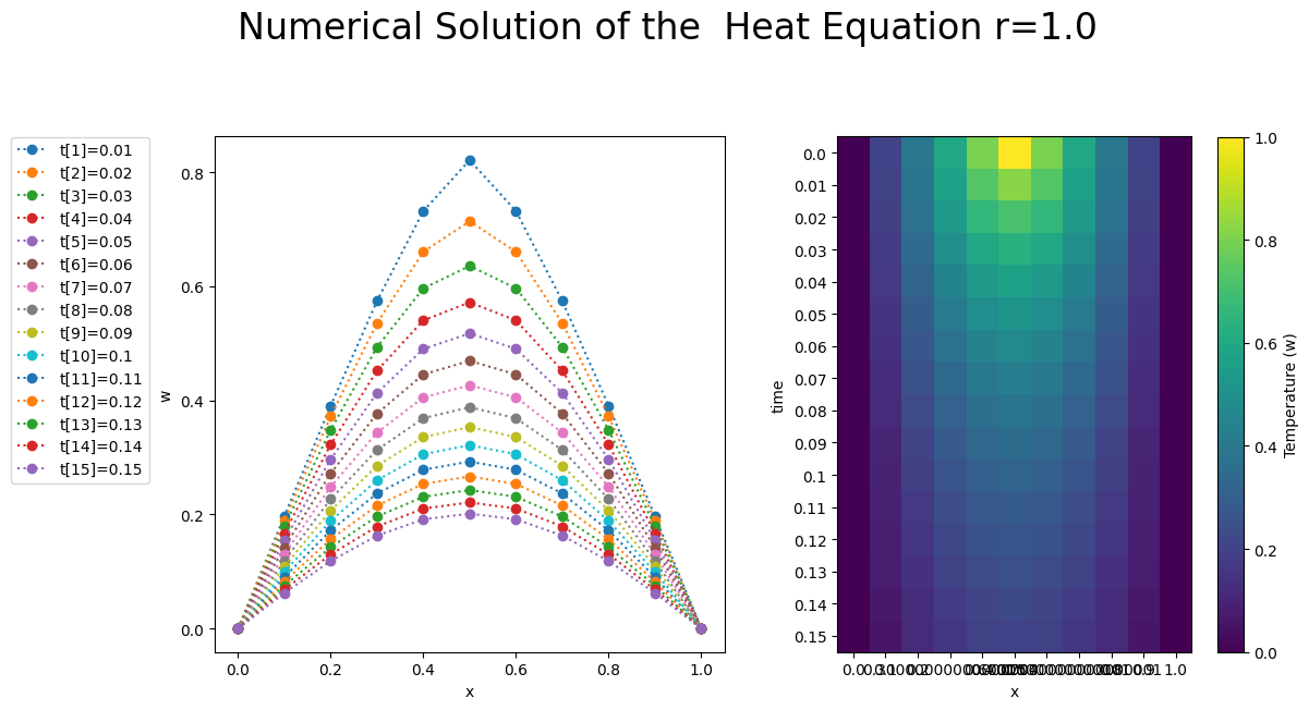
Each set of numerical solutions \(w[i,j]\) for all \(i\) at the previous time step is used to approximate the solution \(w[i,j+1]\). The Figure below shows the numerical approximation \(w[i,j]\) of the Heat Equation using the FTCS method at \(x[i]\) for \(i=0,...,10\) and time steps \(t[j]\) for \(j=1,...,15\). The left plot shows the numerical approximation \(w[i,j]\) as a function of \(x[i]\) with each color representing the different time steps \(t[j]\). The right plot shows the numerical approximation \(w[i,j]\) as colour plot as a function of \(x[i]\), on the \(x[i]\) axis and time \(t[j]\) on the \(y\) axis. The solution is stable for \(r>\frac{1}{2}\) unlike in the explicit method.

fig = plt.figure(figsize=(12,6))

plt.subplot(121)
for j in range (1,time_steps+1):
    b[0]=r*w[0,j]
    b[N-2]=r*w[N,j]
    w[1:(N),j]=np.dot(Ainv,w[1:(N),j-1]+b)
    plt.plot(x,w[:,j],'o:',label='t[%s]=%s'%(j,time[j]))
plt.xlabel('x')
plt.ylabel('w')
#plt.legend(loc='bottom', bbox_to_anchor=(0.5, -0.1))
plt.legend(bbox_to_anchor=(-.4, 1), loc=2, borderaxespad=0.)

plt.subplot(122)
plt.imshow(w.transpose())
plt.xticks(np.arange(len(x)), x)
plt.yticks(np.arange(len(time)), time)
plt.xlabel('x')
plt.ylabel('time')
clb=plt.colorbar()
clb.set_label('Temperature (w)')
plt.suptitle('Numerical Solution of the  Heat Equation r=%s'%(np.round(r,3)),fontsize=24,y=1.08)
fig.tight_layout()
plt.show()

Local Trunction Error

The local truncation error of the classical implicit difference given by

(582)\[\begin{equation} F_{ij+1}(w)=\frac{w_{ij+1}-w_{ij}}{k}-\frac{w_{i+1j+1}-2w_{ij+1}+w_{i-1j+1}}{h^2}=0, \end{equation}\]

of the heat equation

(583)\[\begin{equation} \frac{\partial U}{\partial t} - \frac{\partial^2 U}{\partial x^2}=0, \end{equation}\]

is calculated by substituting the exact solution into the difference scheme give the truncation error:

(584)\[\begin{equation} T_{ij+1}=F_{ij+1}(U)=\frac{U_{ij+1}-U_{ij}}{k}-\frac{U_{i+1j+1}-2U_{ij+1}+U_{i-1j+1}}{h^2}. \end{equation}\]

By Taylors expansions we have

\[\begin{eqnarray*} U_{i+1j}&=&U((i+1)h,(j+1)k)=U(x_i+h,t_{j+1})\\ &=&U_{ij+1}+h\left(\frac{\partial U}{\partial x} \right)_{ij+1}+\frac{h^2}{2}\left(\frac{\partial^2 U}{\partial x^2} \right)_{ij+1}+\frac{h^3}{6}\left(\frac{\partial^3 U}{\partial x^3} \right)_{ij+1} +...\\ U_{i-1j}&=&U((i-1)h,(j+1)k)=U(x_i-h,t_{j+1})\\ &=&U_{ij+1}-h\left(\frac{\partial U}{\partial x} \right)_{ij+1}+\frac{h^2}{2}\left(\frac{\partial^2 U}{\partial x^2} \right)_{ij+1}-\frac{h^3}{6}\left(\frac{\partial^3 U}{\partial x^3} \right)_{ij+1} +...\\ U_{ij}&=&U(ih,(j)k)=U(x_i,t_j)\\ &=&U_{ij+1}-k\left(\frac{\partial U}{\partial t} \right)_{ij+1}+\frac{k^2}{2}\left(\frac{\partial^2 U}{\partial t^2} \right)_{ij+1}-\frac{k^3}{6}\left(\frac{\partial^3 U}{\partial t^3} \right)_{ij+1} +... \end{eqnarray*}\]

substituting these into the expression for \(T_{ij+1}\) gives

\[\begin{eqnarray*} T_{ij+1}&=&\left(\frac{\partial U}{\partial t} - \frac{\partial^2 U}{\partial x^2} \right)_{ij+1}+\frac{k}{2}\left(\frac{\partial^2 U}{\partial t^2} \right)_{ij+1} -\frac{h^2}{12}\left(\frac{\partial^4 U}{\partial x^4} \right)_{ij+1}\\ & & +\frac{k^2}{6}\left(\frac{\partial^3 U}{\partial t^3} \right)_{ij+1} -\frac{h^4}{360}\left(\frac{\partial^6 U}{\partial x^6} \right)_{ij+1}+ \cdots . \end{eqnarray*}\]

As \(U\) is the solution to the differential equation so

(585)\[\begin{equation} \left(\frac{\partial U}{\partial t} - \frac{\partial^2 U}{\partial x^2} \right)_{ij+1}=0,\end{equation}\]

the principal part of the local truncation error is

(586)\[\begin{equation} \frac{k}{2}\left(\frac{\partial^2 U}{\partial t^2} \right)_{ij+1}-\frac{h^2}{12}\left(\frac{\partial^4 U}{\partial x^4} \right)_{ij+1}. \end{equation}\]

Hence the truncation error is

(587)\[\begin{equation} T_{ij}=O(k)+O(h^2). \end{equation}\]

Stability Analysis

To investigating the stability of the fully implicit BTCS difference method of the Heat Equation, we will use the von Neumann method. The difference equation is:

(588)\[\begin{equation}\frac{1}{k}(w_{pq+1}-w_{pq})=\frac{1}{h_x^2}(w_{p-1q+1}-2w_{pq+1}+w_{p+1q+1}),\end{equation}\]

approximating

(589)\[\begin{equation}\frac{\partial U}{\partial t}=\frac{\partial^2 U}{\partial x^2}\end{equation}\]

at \((ph,k(q+1))\). Substituting \(w_{pq}=e^{i\beta x}\xi^{q}\) into the difference equation gives:

(590)\[\begin{equation}e^{i\beta ph}\xi^{q+1}-e^{i\beta ph}\xi^{q}=r\{e^{i\beta (p-1)h}\xi^{q+1}-2e^{i\beta ph}\xi^{q+1}+e^{i\beta (p+1)h}\xi^{q+1} \} \end{equation}\]

where \(r=\frac{k}{h_x^2}\). Divide across by \(e^{i\beta (p)h}\xi^{q}\) leads to

(591)\[\begin{equation} \xi-1=r \xi (e^{i\beta (-1)h} -2+e^{i\beta h}), \end{equation}\]

(592)\[\begin{equation}\xi-\xi r (2\cos(\beta h)-2)= 1,\end{equation}\]

(593)\[\begin{equation}\xi(1+4r\sin^2(\beta\frac{h}{2})) =1.\end{equation}\]

Hence

(594)\[\begin{equation}\xi=\frac{1}{(1+4r\sin^2(\beta\frac{h}{2}))} \leq 1\end{equation}\]

therefore the equation is unconditionally stable as \(0 < \xi \leq 1\) for all \(r\) and all \(\beta\) .

References

[1] G D Smith Numerical Solution of Partial Differential Equations: Finite Difference Method Oxford 1992

[2] Butler, J. (2019). John S Butler Numerical Methods for Differential Equations. [online] Maths.dit.ie. Available at: http://www.maths.dit.ie/~johnbutler/Teaching_NumericalMethods.html [Accessed 14 Mar. 2019].

[3] Wikipedia contributors. (2019, February 22). Heat equation. In Wikipedia, The Free Encyclopedia. Available at: https://en.wikipedia.org/w/index.php?title=Heat_equation&oldid=884580138 [Accessed 14 Mar. 2019].