Consistency of a Multistep method

Consistency of a Multistep method#

John S Butler#

john.s.butler@tudublin.ie
Course Notes Github

Overview#

A one-step or multistep method is used to approximate the solution of an initial value problem of the form

(322)#\[\begin{equation} \frac{dy}{dt}=f(t,y), \end{equation}\]

with the initial condition

(323)#\[\begin{equation} y(a)=\alpha.\end{equation}\]

The method should only be used if it satisfies the three criteria:

that difference equation is consistent with the differential equation;
that the numerical solution is convergent to the exact answer of the differential equation;
that the numerical solution is stable.

In the notebooks in this folder we will illustate examples of consisten and inconsistent, convergent and non-convergent, and stable and unstable methods.

Introduction to Consistency#

In this notebook we will illustate an inconsistent method.

from IPython.display import HTML
HTML('<iframe width="560" height="315" src="https://www.youtube.com/embed/SXH6WHMLTII" frameborder="0" allow="accelerometer; autoplay; clipboard-write; encrypted-media; gyroscope; picture-in-picture" allowfullscreen></iframe>')

/Users/johnbutler/opt/anaconda3/lib/python3.8/site-packages/IPython/core/display.py:724: UserWarning: Consider using IPython.display.IFrame instead
  warnings.warn("Consider using IPython.display.IFrame instead")

Definition#

A one-step and multi-step methods with local truncation error $\tau_{i}(h)$ at the $i$th step is said to be consistent with the differential equation it approximates if

(324)#\[\begin{equation}\lim_{h \rightarrow 0} (\max_{1 \leq i \leq N}|\tau_{i}(h)|)=0 \end{equation}\]

where

(325)#\[\begin{equation}\tau_{i}(h)=\frac{y_{i+1}-y_{i}}{h}-F(t_i,y_i,h,f) \end{equation}\]

As $h \rightarrow 0$ does $F(t_i,y_i,h,f) \rightarrow f(t,y)$.

All the Runge Kutta, and Adams methods are consistent in this course. This notebook will illustrate a non-consistent method which with great hubris I will call the Abysmal-Butler methods.

2-step Abysmal Butler Method#

The 2-step Abysmal Butler difference equation is given by

(326)#\[\begin{equation}w_{i+1} = w_{i} + \frac{h}{2}(4f(t_i,w_i)-3f(t_{i-1},w_{i-1})), \end{equation}\]

which can be written as

(327)#\[\begin{equation}\frac{w_{i+1} -w_{i}}{h} = \frac{1}{2}(4f(t_i,w_i)-3f(t_{i-1},w_{i-1})). \end{equation}\]

Intial Value Problem#

To illustrate consistency we will apply the method to a linear intial value problem given by

(328)#\[\begin{equation} y^{'}=t-y, \ \ (0 \leq t \leq 2),\end{equation}\]

with the initial condition

(329)#\[\begin{equation}y(0)=1,\end{equation}\]

with the exact solution

(330)#\[\begin{equation}y(t)= 2e^{-t}+t-1.\end{equation}\]

Python Libraries#

import numpy as np
import math 
import pandas as pd

%matplotlib inline
import matplotlib.pyplot as plt # side-stepping mpl backend
import matplotlib.gridspec as gridspec # subplots
import warnings
warnings.filterwarnings("ignore")

Defining the function#

$$ f(t,y)=t-y.\end{equation}

def myfun_ty(t,y):
    return t-y

Discrete Interval#

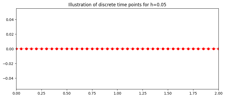
Defining the step size $h$ from the interval range $a \leq t\leq b$ and number of steps $N$

(331)#\[\begin{equation}h=\frac{b - a}{N}.\end{equation}\]

This gives the discrete time steps,

(332)#\[\begin{equation}t_i=t_0+ih,\end{equation}\]

where $t_0=a.$

Here the interval is $0\leq t \leq 2$ and number of step 40

(333)#\[\begin{equation}h=\frac{2−0}{40}=0.05.\end{equation}\]

This gives the discrete time steps,

(334)#\[\begin{equation}t_i=0+i0.5,\end{equation}\]

for $i=0,1,⋯,40.$

# Start and end of interval
b=2
a=0
# Step size
N=40
h=(b-a)/(N)
t=np.arange(a,b+h,h)
fig = plt.figure(figsize=(10,4))
plt.plot(t,0*t,'o:',color='red')
plt.xlim((0,2))
plt.title('Illustration of discrete time points for h=%s'%(h))
plt.show()

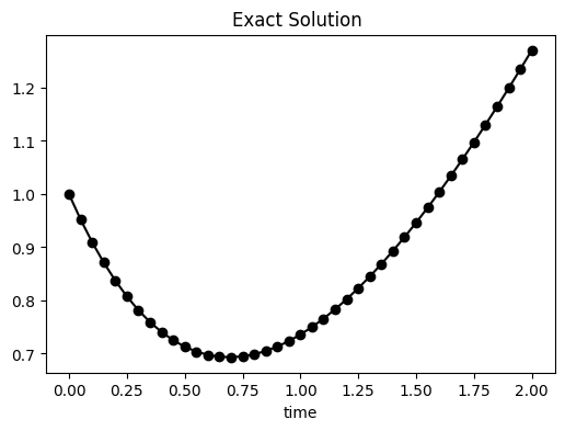
../_images/3415bfc1c372f2da12f34f1a7a6d432af70eb78e4f0609b92efaab56a8504cc9.png

Exact Solution#

The initial value problem has the exact solution $$y(t)=2e^{-t}+t-1.\end{equation} The figure below plots the exact solution.

IC=1 # Intial condtion
y=(IC+1)*np.exp(-t)+t-1
fig = plt.figure(figsize=(6,4))
plt.plot(t,y,'o-',color='black')
plt.title('Exact Solution ')
plt.xlabel('time')
plt.show()

../_images/cac0f21882d3cf855bf6c9aeb9b68a1a37c89e483c7f64755ed4ad3bc50dac9f.png

# Initial Condition
w=np.zeros(N+1)
#np.zeros(N+1)
w[0]=IC

2-step Abysmal Butler Method#

The 2-step Abysmal Butler difference equation is

(335)#\[\begin{equation}w_{i+1} = w_{i} + \frac{h}{2}(4f(t_i,w_i)-3f(t_{i-1},w_{i-1})).\end{equation}\]

For $i=0$ the system of difference equation is:

(336)#\[\begin{equation}w_{1} = w_{0} + \frac{h}{2}(4(t_0-w_0)-3(t_{-1}-w_{-1})) \end{equation}\]

this is not solvable as $w_{-1}$ is unknown.

For $i=1$ the difference equation is:

(337)#\[\begin{equation}w_{2} = w_{1} + \frac{h}{2}(4(t_1-w_1)-3(t_{0}-w_{0})),\end{equation}\]

this is not solvable as $w_{1}$ is unknown. $w_1$ can be approximated using a one step method. Here, as the exact solution is known,

(338)#\[\begin{equation}w_1=2e^{-t_1}+t_1-1.\end{equation}\]

### Initial conditions
w=np.zeros(len(t))
w0=np.zeros(len(t))
w[0]=IC
w[1]=y[1]

Loop#

for k in range (1,N):
    w[k+1]=(w[k]+h/2.0*(4*myfun_ty(t[k],w[k])-3*myfun_ty(t[k-1],w[k-1])))   

Plotting solution#

def plotting(t,w,y):
    fig = plt.figure(figsize=(10,4))
    plt.plot(t,y, 'o-',color='black',label='Exact')
    plt.plot(t,w,'^:',color='red',label='Abysmal-Butler')
    plt.xlabel('time')
    plt.legend()
    plt.show 

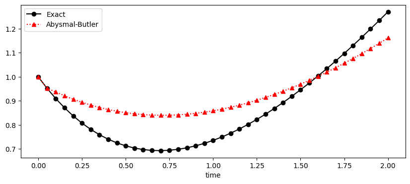
The plot below shows the exact solution (black) and the Abysmal-Butler approximation (red) of the intial value problem.

The Numerical approximation does not do a good job of approximating the exact solution and that is because it is inconsistent.

plotting(t,w,y)

../_images/dd8aa5876afe6831670c5fa8c26b745ce080be1ea365afeef5c91b1cd7f73802.png

Consistency#

To prove that the Abysmal-Butler method does not satisfy the consistency condition,

(339)#\[\begin{equation} \tau_{i}(h)=\frac{y_{i+1}-y_{i}}{h}-\frac{1}{2}[4(f(t_i,y_i)-3f(t_{i-1},y_{i-1})]. \end{equation}\]

As $h \rightarrow 0$

(340)#\[\begin{equation} \frac{1}{2}[4f(t_i,y_i)-3f(t_{i-1},y_{i-1})] \rightarrow \frac{f(t_i,y_i)}{2}.\end{equation}\]

While as $h \rightarrow 0$

(341)#\[\begin{equation} \frac{y_{i+1}-y_{i}}{h} \rightarrow y^{'}=f(t_i,y_i).\end{equation}\]

Hence as $h \rightarrow 0$ \begin{equation} \frac{y_{i+1}-y_{i}}{h}-\frac{1}{2}[4(f(t_i,y_i)-3f(t_{i-1},y_{i-1})]\rightarrow f(t_i,y_i)-\frac{f(t_i,y_i)}{2}=\frac{f(t_i,y_i)}{2},\end{equation} which violates the consistency condition (inconsistent).

d = {'time': t[0:5], 'Abysmal Butler': w[0:5],'Exact':y[0:5],'Error':np.abs(y[0:5]-w[0:5])}
df = pd.DataFrame(data=d)
df

	time	Abysmal Butler	Exact	Error
0	0.00	1.000000	1.000000	0.000000
1	0.05	0.952459	0.952459	0.000000
2	0.10	0.937213	0.909675	0.027538
3	0.15	0.921176	0.871416	0.049760
4	0.20	0.906849	0.837462	0.069388

Consistency of a Multistep method

Contents

Consistency of a Multistep method#

John S Butler#

Overview#

Introduction to Consistency#

Definition#

2-step Abysmal Butler Method#

Intial Value Problem#

Python Libraries#

Defining the function#

Discrete Interval#

Exact Solution#

2-step Abysmal Butler Method#

Loop#

Plotting solution#

Consistency#