Linear Shooting Method

Linear Shooting Method#

John S Butler john.s.butler@tudublin.ie Course Notes Github #

Overview#

This notebook illustates the implentation of a linear shooting method to a linear boundary value problem. The video below walks through the code.

from IPython.display import HTML
HTML('<iframe width="560" height="315" src="https://www.youtube.com/embed/g0JrcJVFoZg" frameborder="0" allow="accelerometer; autoplay; clipboard-write; encrypted-media; gyroscope; picture-in-picture" allowfullscreen></iframe>')

/Users/johnbutler/opt/anaconda3/lib/python3.8/site-packages/IPython/core/display.py:724: UserWarning: Consider using IPython.display.IFrame instead
  warnings.warn("Consider using IPython.display.IFrame instead")

Introduction#

To numerically approximate the Boundary Value Problem

(444)#\[\begin{equation} y^{''}=p(x)y^{'}+q(x)y+r(x) \ \ \ a < x < b \end{equation}\]

with the left and right boundary conditions:

(445)#\[\begin{equation}y(a)=\alpha, \end{equation}\]

(446)#\[\begin{equation}y(b) =\beta. \end{equation}\]

The Boundary Value Problem is divided into two Initial Value Problems:

The first 2nd order Initial Value Problem is the same as the original Boundary Value Problem with an extra initial condtion $y_1^{'}(a)=0$.

(447)#\[\begin{equation} y^{''}_1=p(x)y^{'}_1+q(x)y_1+r(x), \ \ y_1(a)=\alpha, \ \ \color{green}{y^{'}_1(a)=0},\\ \end{equation}\]

The second 2nd order Initial Value Problem is the homogenous form of the original Boundary Value Problem, by removing $r(x)$, with the initial condtions $y_2(a)=0$ and $y_2^{'}(a)=1$.

(448)#\[\begin{equation} y^{''}_2=p(x)y^{'}_2+q(x)y_2, \ \ \color{green}{y_2(a)=0, \ \ y^{'}_2(a)=1}. \end{equation}\]

combining these intial values problems together to get the unique solution

(449)#\[\begin{equation} y(x)=y_1(x)+\frac{\beta-y_1(b)}{y_2(b)}y_2(x), \end{equation}\]

provided that $y_2(b)\not=0$.

The truncation error for the shooting method is
$$ |y_i - y(x_i)| \leq K h^n\left|1+\frac{y_{2 i}}{y_{2 i}}\right| $O(h^n)$ is the order of the numerical method used to approximate the solution of the Initial Value Problems.

import numpy as np
import math
import matplotlib.pyplot as plt
import pandas as pd
import warnings
warnings.filterwarnings("ignore")

Example Boundary Value Problem#

To illustrate the shooting method we shall apply it to the Boundary Value Problem:

(450)#\[\begin{equation}y^{''}=2y^{'}+3y-6, \end{equation}\]

with boundary conditions

(451)#\[\begin{equation}y(0) = 3, \end{equation}\]

(452)#\[\begin{equation}y(1) = e^3+2, \end{equation}\]

with the exact solution is

(453)#\[\begin{equation}y=e^{3x}+2. \end{equation}\]

The boundary value problem is broken into two second order Initial Value Problems:

The first 2nd order Intial Value Problem is the same as the original Boundary Value Problem with an extra initial condtion $u^{'}(0)=0$.

(454)#\[\begin{equation} u^{''} =2u'+3u-6, \ \ \ \ u(0)=3, \ \ \ \color{green}{u^{'}(0)=0} \end{equation}\]

The second 2nd order Intial Value Problem is the homogenous form of the original Boundary Value Problem with the initial condtions $w^{'}(0)=0$ and $w^{'}(0)=1$.

(455)#\[\begin{equation} w^{''} =2w^{'}+3w, \ \ \ \ \color{green}{w(0)=0}, \ \ \ \color{green}{w^{'}(0)=1} \end{equation}\]

combining these results of these two intial value problems as a linear sum

(456)#\[\begin{equation} y(x)=u(x)+\frac{e^{3x}+2-u(1)}{w(1)}w(x) \end{equation}\]

gives the solution of the Boundary Value Problem.

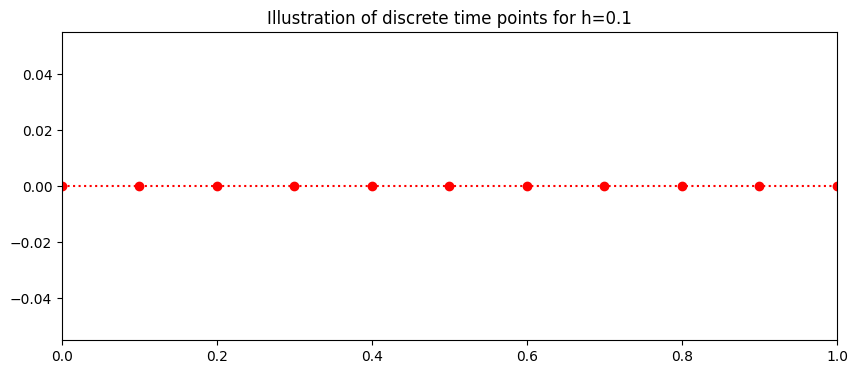
Discrete Axis#

The stepsize is defined as

(457)#\[\begin{equation}h=\frac{b-a}{N}, \end{equation}\]

here it is

(458)#\[\begin{equation}h=\frac{1-0}{10}, \end{equation}\]

giving

(459)#\[\begin{equation}x_i=0+0.1 i, \end{equation}\]

for $i=0,1,...10.$

## BVP
N=10
h=1/N
x=np.linspace(0,1,N+1)
fig = plt.figure(figsize=(10,4))
plt.plot(x,0*x,'o:',color='red')
plt.xlim((0,1))
plt.title('Illustration of discrete time points for h=%s'%(h))

plt.show()

../_images/5649eda549dd65a3b6d98978d7d11bf70753403c0ec4ed43271c6b548f7955c5.png

Initial conditions#

The initial conditions for the discrete equations are: $$ u_1[0]=3$$ \color{green}{u_2[0]=0}$$ \color{green}{w_1[0]=0}$$ \color{green}{w_2[0]=1}$$

U1=np.zeros(N+1)
U2=np.zeros(N+1)
W1=np.zeros(N+1)
W2=np.zeros(N+1)

U1[0]=3
U2[0]=0

W1[0]=0
W2[0]=1

Numerical method#

The Euler method is applied to numerically approximate the solution of the system of the two second order initial value problems they are converted in to two pairs of two first order initial value problems:

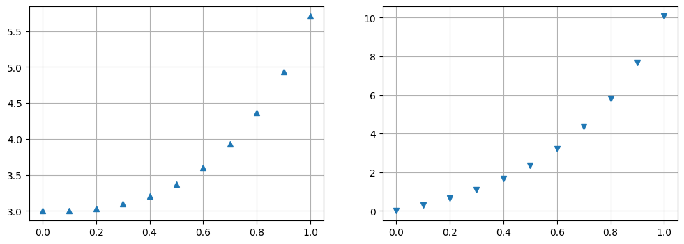
1. Inhomogenous Approximation#

The plot below shows the numerical approximation for the two first order Intial Value Problems

(460)#\[\begin{equation} u_1^{'} =u_2, \ \ \ \ u_1(0)=3, \end{equation}\]

(461)#\[\begin{equation} u_2^{'} =2u_2+3u_1-6, \ \ \ \color{green}{u_2(0)=0}, \end{equation}\]

that Euler approximate of the inhomogeneous two Initial Value Problems is :

(462)#\[\begin{equation}u_{1}[i+1]=u_{1}[i] + h u_{2}[i] \end{equation}\]

(463)#\[\begin{equation}u_{2}[i+1]=u_{2}[i] + h (2u_{2}[i]+3u_{1}[i] -6) \end{equation}\]

with $u_1[0]=3$ and $\color{green}{u_2[0]=0}$.

for i in range (0,N):
    U1[i+1]=U1[i]+h*(U2[i])
    U2[i+1]=U2[i]+h*(2*U2[i]+3*U1[i]-6)

Plots#

The plot below shows the Euler approximation of the two intial value problems $u_1$ on the left and $u2$ on the right.

fig = plt.figure(figsize=(12,4))
ax = fig.add_subplot(1,2,1)
plt.plot(x,U1,'^')
#plt.title(r"$u_1'=u_2, \ \  u_1(0)=3$",fontsize=16)
plt.grid(True)

ax = fig.add_subplot(1,2,2)
plt.plot(x,U2,'v')
#plt.title("U2", fontsize=16)

plt.grid(True)
plt.show()

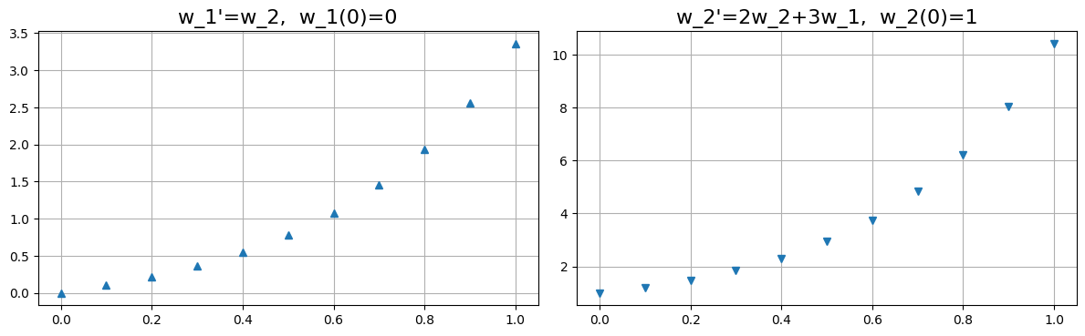
../_images/be9ff34303bb74002f396b06e40dccf4b6aa8ba009552ab638cd203e20c032bf.png

2. Homogenous Approximation#

The homogeneous Bounday Value Problem is divided into two first order Intial Value Problems

(464)#\[\begin{equation} w_1^{'} =w_2, \ \ \ \ \color{green}{w_1(0)=0} \end{equation}\]

(465)#\[\begin{equation} w_2^{'} =2w_2+3w_1, \ \ \ \color{green}{w_2(0)=1} \end{equation}\]

The Euler approximation of the homogeneous of the two Initial Value Problem is

(466)#\[\begin{equation}w_{1}[i+1]=w_{1}[i] + h w_{2}[i] \end{equation}\]

(467)#\[\begin{equation}w_{2}[i+1]=w_{2}[i] + h (2w_{2}[i]+3w_{1}[i]) \end{equation}\]

with $\color{green}{w_1[0]=0}$ and $\color{green}{w_2[0]=1}$.

for i in range (0,N):
    W1[i+1]=W1[i]+h*(W2[i])
    W2[i+1]=W2[i]+h*(2*W2[i]+3*W1[i])

Homogenous Approximation#

Plots#

The plot below shows the Euler approximation of the two intial value problems $u_1$ on the left and $u2$ on the right.

fig = plt.figure(figsize=(12,4))
ax = fig.add_subplot(1,2,1)
plt.plot(x,W1,'^')
plt.grid(True)
plt.title("w_1'=w_2,  w_1(0)=0",fontsize=16)

ax = fig.add_subplot(1,2,2)
plt.plot(x,W2,'v')
plt.grid(True)
plt.title("w_2'=2w_2+3w_1,  w_2(0)=1",fontsize=16)
plt.tight_layout()
plt.subplots_adjust(top=0.85)

plt.show()
beta=math.exp(3)+2
y=U1+(beta-U1[N])/W1[N]*W1

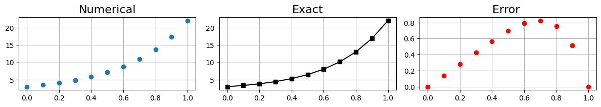
../_images/8aa3f20362d308c2e55faf272d333f93698d1ecc4d3703c0f525dd6490336d03.png

Approximate Solution#

Combining together the numerical approximation of $u_1$ and $w_1$ as a weighted sum

(468)#\[\begin{equation}y(x[i])\approx u_{1}[i] + \frac{e^3+2-u_{1}[N]}{w_1[N]}w_{1}[i] \end{equation}\]

gives the approximate solution of the Boundary Value Problem.

The truncation error for the shooting method using the Euler method is

(469)#\[\begin{equation} |y_i - y(x[i])| \leq K h\left|1+\frac{w_{1}[i]}{u_{1}[i]}\right| \end{equation}\]

$O(h)$ is the order of the method.

The plot below shows the approximate solution of the Boundary Value Problem (left), the exact solution (middle) and the error (right)

Exact=np.exp(3*x)+2
fig = plt.figure(figsize=(12,4))
ax = fig.add_subplot(2,3,1)
plt.plot(x,y,'o')

plt.grid(True)
plt.title("Numerical",
          fontsize=16)

ax = fig.add_subplot(2,3,2)
plt.plot(x,Exact,'ks-')

plt.grid(True)
plt.title("Exact",
          fontsize=16)

ax = fig.add_subplot(2,3,3)
plt.plot(x,abs(y-Exact),'ro')
plt.grid(True)
plt.title("Error ",fontsize=16)
          
plt.tight_layout()
plt.subplots_adjust(top=0.85)
plt.show()

../_images/36da14d5c3eb4770e606433d1fde96c7578482d497902fa5fd426691db53fc71.png

Data#

The Table below shows that output for $x$, the Euler numerical approximations $U1$, $U2$, $W1$ and $W2$ of the system of four Intial Value Problems, the shooting methods approximate solution $y_i=u_{1 i} + \frac{e^3+2-u_{1}(x_N)}{w_1(x_N)}w_{1 i}$ and the exact solution of the Boundary Value Problem.

d = {'time x_i': x[0:10], 
     'U1':np.round(U1[0:10],3),
     'U2':np.round(U2[0:10],3),
     'W1':np.round(W1[0:10],3),
     'W2':np.round(W2[0:10],3),
     'y_i':np.round(W2[0:10],3),
     'y(x_i)':np.round(W2[0:10],3)
    }
df = pd.DataFrame(data=d)
df

	time x_i	U1	U2	W1	W2	y_i	y(x_i)
0	0.0	3.000	0.000	0.000	1.000	1.000	1.000
1	0.1	3.000	0.300	0.100	1.200	1.200	1.200
2	0.2	3.030	0.660	0.220	1.470	1.470	1.470
3	0.3	3.096	1.101	0.367	1.830	1.830	1.830
4	0.4	3.206	1.650	0.550	2.306	2.306	2.306
5	0.5	3.371	2.342	0.781	2.932	2.932	2.932
6	0.6	3.605	3.222	1.074	3.753	3.753	3.753
7	0.7	3.927	4.347	1.449	4.826	4.826	4.826
8	0.8	4.362	5.795	1.932	6.226	6.226	6.226
9	0.9	4.942	7.663	2.554	8.050	8.050	8.050

Linear Shooting Method

Contents

Linear Shooting Method#

John S Butler john.s.butler@tudublin.ie Course Notes Github#

Overview#

Introduction#

Example Boundary Value Problem#

Discrete Axis#

Initial conditions#

Numerical method#

1. Inhomogenous Approximation#

Plots#

2. Homogenous Approximation#

Homogenous Approximation#

Plots#

Approximate Solution#

Data#

John S Butler john.s.butler@tudublin.ie Course Notes Github #