Finite Difference Method

John S Butler john.s.butler@tudublin.ie Course Notes Github

Overview

This notebook illustrates the finite different method for a linear Boundary Value Problem.

Example 2 Boundary Value Problem

To further illustrate the method we will apply the finite difference method to the this boundary value problem

(530)\[\begin{equation} \frac{d^2 y}{dx^2} + 2x\frac{dy}{dx}+y=3x^2,\end{equation}\]

with the boundary conditions

(531)\[\begin{equation} y(0)=1, y(1)=2. \end{equation}\]

import numpy as np
import math
import matplotlib.pyplot as plt

Discrete Axis

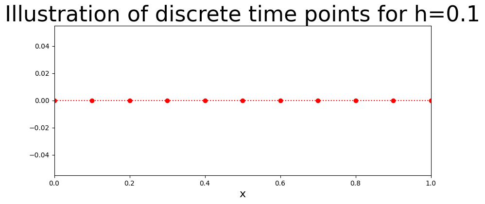
The stepsize is defined as

(532)\[\begin{equation}h=\frac{b-a}{N}\end{equation}\]

here it is

(533)\[\begin{equation}h=\frac{1-0}{10}\end{equation}\]

giving

(534)\[\begin{equation}x_i=0+0.1 i\end{equation}\]

for \(i=0,1,...10.\)

## BVP
N=10
h=1/N
x=np.linspace(0,1,N+1)
fig = plt.figure(figsize=(10,4))
plt.plot(x,0*x,'o:',color='red')
plt.xlim((0,1))
plt.xlabel('x',fontsize=16)
plt.title('Illustration of discrete time points for h=%s'%(h),fontsize=32)
plt.show()

The Difference Equation

To convert the boundary problem into a difference equation we use 1st and 2nd order difference operators.

The first derivative can be approximated by the difference operators:

(535)\[\begin{equation}D^{+}U_{i}=\frac{U_{i+1}-U_{i}}{h_{i+1}} \ \ \ \mbox{ Forward,} \end{equation}\]

(536)\[\begin{equation}D^{-}U_{i}=\frac{U_{i}-U_{i-1}}{h_i} \ \ \ \mbox{ Backward,} \end{equation}\]

or

(537)\[\begin{equation}D^{0}U_{i}=\frac{U_{i+1}-U_{i-1}}{x_{i+1}-x_{i-1}} \ \ \ \mbox{ Centered.} \end{equation}\]

The second derivative can be approxiamed

(538)\[\begin{equation}\delta_x^{2}U_{i}=\frac{2}{x_{i+1}-x_{i-1}}\left(\frac{U_{i+1}-U_{i}}{x_{i+1}-x_{i}}-\frac{U_{i}-U_{i-1}}{x_{i}-x_{i-1}}\right) \ \ \ \mbox{ Centered in $x$ direction} \end{equation}\]

Given the differential equation

(539)\[\begin{equation} \frac{d^2 y}{dx^2} + 2x\frac{dy}{dx}+y=3x^2,\end{equation}\]

the difference equation is,

(540)\[\begin{equation}\frac{1}{h^2}\left(y_{i-1}-2y_i+y_{i+1}\right)+2x_i\frac{y_{i+1}-y_{i-1}}{2h}+y_i=3x^2_i \ \ \ i=1,..,N-1. \end{equation}\]

Rearranging the equation we have the system of N-1 equations

(541)\[\begin{equation}i=1: (\frac{1}{0.1^2}-\frac{2x_1}{0.2})\color{green}{y_{0}} -\left(\frac{2}{0.1^2}-1\right)y_1 +(\frac{1}{0.1^2}+\frac{2x_1}{0.2}) y_{2}=3x_1^2\end{equation}\]

(542)\[\begin{equation}i=2: (\frac{1}{0.1^2}-\frac{2x_2}{0.2})y_{1} -\left(\frac{2}{0.1^2}-1\right)y_2 +(\frac{1}{0.1^2}+\frac{2x_2}{0.2}) y_{3}=3x_2^2\end{equation}\]

(543)\[\begin{equation} ...\end{equation}\]

(544)\[\begin{equation}i=8: (\frac{1}{0.1^2}-\frac{2x_8}{0.2})y_{7} -\left(\frac{2}{0.1^2}-1\right)y_8 +(\frac{1}{0.1^2}+\frac{2x_8}{0.2})y_{9}=3x_8^2\end{equation}\]

(545)\[\begin{equation}i=9: (\frac{1}{0.1^2}-\frac{2x_9}{0.2})y_{8} -\left(\frac{2}{0.1^2}-1\right)y_9 +(\frac{1}{0.1^2}+\frac{2x_9}{0.2}) \color{green}{y_{10}}=3x_9^2\end{equation}\]

where the green terms are the known boundary conditions.

Rearranging the equation we have the system of 9 equations

(546)\[\begin{equation}i=1: -\left(\frac{2}{0.1^2}-1\right)y_1 +(\frac{1}{0.1^2}+\frac{2x_1}{0.2})y_{2}=-(\frac{1}{0.1^2}-\frac{2x_1}{0.2})\color{green}{y_{0}}+3x_1^2\end{equation}\]

(547)\[\begin{equation}i=2: (\frac{1}{0.1^2}-\frac{2x_2}{0.2})y_{1} -\left(\frac{2}{0.1^2}-1\right)y_2 +(\frac{1}{0.1^2}+\frac{2x_2}{0.2}) y_{3}=3x_2^2\end{equation}\]

(548)\[\begin{equation} ...\end{equation}\]

(549)\[\begin{equation}i=8: (\frac{1}{0.1^2}-\frac{2x_8}{0.2})y_{7} -\left(\frac{2}{0.1^2}-1\right)y_8 +(\frac{1}{0.1^2}+\frac{2x_8}{0.2}) y_{9}=3x_8^2\end{equation}\]

(550)\[\begin{equation}i=9: (\frac{1}{0.1^2}-\frac{2x_9}{0.2})y_{8} -\left(\frac{2}{0.1^2}-1\right)y_9 =-(\frac{1}{0.1^2}+\frac{2x_9}{0.2}) \color{green}{y_{10}}+3x_9^2\end{equation}\]

where the green terms are the known boundary conditions. This is system can be put into matrix form

(551)\[\begin{equation} A\color{red}{\mathbf{y}}=\mathbf{b} \end{equation}\]

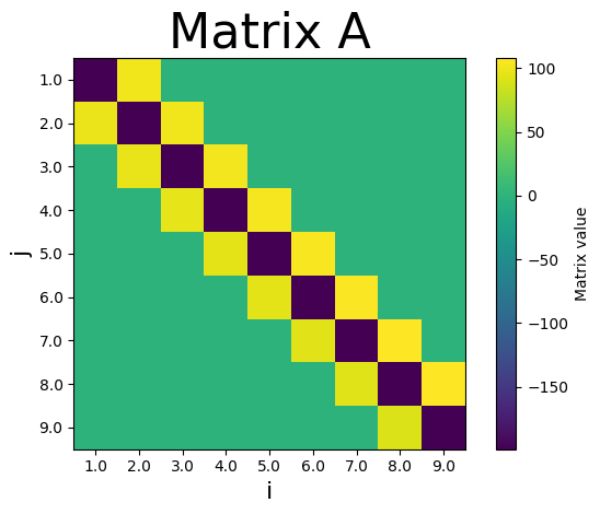
Where A is a \(9\times 9 \) matrix of the form

which can be represented graphically as:

A=np.zeros((N-1,N-1))
# Diagonal
for i in range (0,N-1):
    A[i,i]=-(2/(h*h)-1) # Diagonal

for i in range (0,N-2):           
    A[i+1,i]=1/(h*h)-2*(i+1)*h/(2*h) ## Lower Diagonal
    A[i,i+1]=1/(h*h)+2*(i+1)*h/(2*h) ## Upper Diagonal
    
plt.imshow(A)
plt.xlabel('i',fontsize=16)
plt.ylabel('j',fontsize=16)
plt.yticks(np.arange(N-1), np.arange(1,N-0.9,1))
plt.xticks(np.arange(N-1), np.arange(1,N-0.9,1))
clb=plt.colorbar()
clb.set_label('Matrix value')
plt.title('Matrix A',fontsize=32)
plt.tight_layout()
plt.subplots_adjust()
plt.show()

\(\mathbf{y}\) is the unknown vector which is contains the numerical approximations of the \(y\).

(552)\[\begin{equation} \color{red}{\mathbf{y}}=\color{red}{ \left(\begin{array}{c} y_1\\ y_2\\ y_3\\ .\\ .\\ y_8\\ y_9 \end{array}\right).} \end{equation}\]

y=np.zeros((N+1))
# Boundary Condition
y[0]=1
y[N]=2

and the known right hand side is a known \(9\times 1\) vector with the boundary conditions

(553)\[\begin{equation} \mathbf{b}=\left(\begin{array}{c}-99+3x_1^2\\ 3x_2^2\\ 3x_3^2\\ .\\ .\\ 3x_8^2\\ -209+3x_9^2 \end{array}\right) \end{equation}\]

b=np.zeros(N-1)
for i in range (0,N-1):
    b[i]=3*h*(i+1)*h*(i+1)
# Boundary Condition
b[0]=-y[0]*(1/(h*h)-2*1*h/(2*h))+b[0]
b[N-2]=-y[N]*(1/(h*h)+2*9*h/(2*h))+b[N-2]
print('b=')
print(b)

b=
[-9.8970e+01  1.2000e-01  2.7000e-01  4.8000e-01  7.5000e-01  1.0800e+00
  1.4700e+00  1.9200e+00 -2.1557e+02]

Solving the system

To solve invert the matrix \(A\) such that

(554)\[\begin{equation}A^{-1}Ay=A^{-1}b\end{equation}\]

(555)\[\begin{equation}y=A^{-1}b\end{equation}\]

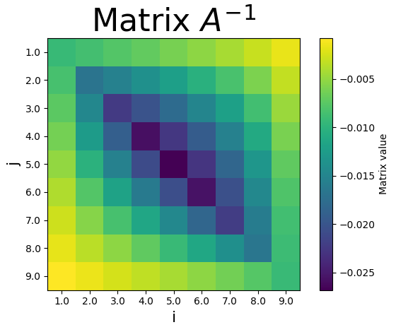
The plot below shows the graphical representation of \(A^{-1}\).

invA=np.linalg.inv(A)

plt.imshow(invA)
plt.xlabel('i',fontsize=16)
plt.ylabel('j',fontsize=16)
plt.yticks(np.arange(N-1), np.arange(1,N-0.9,1))
plt.xticks(np.arange(N-1), np.arange(1,N-0.9,1))
clb=plt.colorbar()
clb.set_label('Matrix value')
plt.title(r'Matrix $A^{-1}$',fontsize=32)
plt.tight_layout()
plt.subplots_adjust()
plt.show()


y[1:N]=np.dot(invA,b)

Result

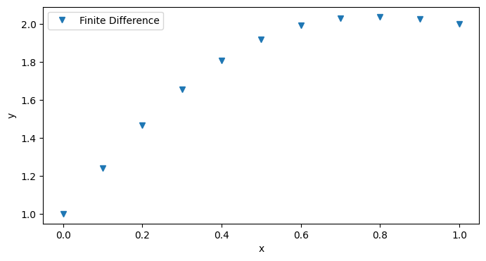
The plot below shows the approximate solution of the Boundary Value Problem (blue v).

fig = plt.figure(figsize=(8,4))

plt.plot(x,y,'v',label='Finite Difference')
plt.xlabel('x')
plt.ylabel('y')
plt.legend(loc='best')
plt.show()