![]()
Taylor Method#
This notebook implements the 3rd order Taylor method for three different population intial value problems.
The Taylor method is derived from the Taylor expansion as depicted by Monica Alexander in the figure below:

3rd Order Taylor#
The general 3rd Order Taylor method for to the first order differential equation
numerical approximates \(y\) the at time point \(t_i\) as \(w_i\) with the formula:
where \(h\) is the stepsize. for \(i=0,...,N-1\). With the local truncation error of
where \(\xi \in [t_i,t_{i+1}]\). To illustrate the method we will apply it to three intial value problems:
1. Linear#
Consider the linear population Differential Equation
with the initial condition,
2. Non-Linear Population Equation#
Consider the non-linear population Differential Equation
with the initial condition,
3. Non-Linear Population Equation with an oscillation#
Consider the non-linear population Differential Equation with an oscillation
with the initial condition,
Read in Libraries#
## Library
import numpy as np
import math
import pandas as pd

%matplotlib inline
import matplotlib.pyplot as plt # side-stepping mpl backend
import matplotlib.gridspec as gridspec # subplots
import warnings

warnings.filterwarnings("ignore")
Discrete Interval#
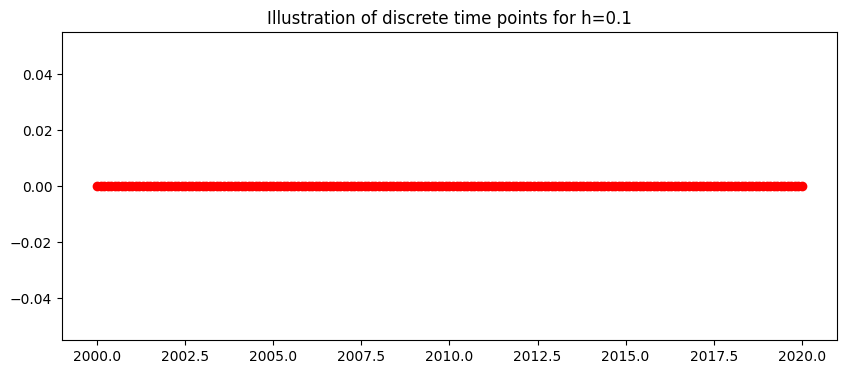
The continuous time \(a\leq t \leq b \) is discretised into \(N\) points seperated by a constant stepsize
Here the interval is \(2000\leq t \leq 2020,\)
This gives the 201 discrete points:
This is generalised to
The plot below shows the discrete time steps:
N=200
t_end=2020.0
t_start=2000.0
h=((t_end-t_start)/N)
t=np.arange(t_start,t_end+h/2,h)
fig = plt.figure(figsize=(10,4))
plt.plot(t,0*t,'o:',color='red')
plt.title('Illustration of discrete time points for h=%s'%(h))
plt.show()
1. Linear Population Equation#
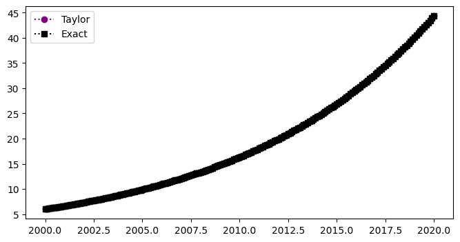
Exact Solution#
The linear population equation
with the initial condition,
has a known exact (analytic) solution
Specific 3rd Order Taylor for the Linear Population Equation#
To write the specific 3rd Order Taylor difference equation for the intial value problem we need to calculate the first derivative of
def linfun(t,w):
    ftw=0.1*w
    return ftw
with respect to \(t\),
def linfun_d(t,w):
    ftw=0.01*w
    return ftw
and the second derivative of \(f\) with respect to \(t\),
def linfun_dd(t,w):
    ftw=0.001*w
    return ftw
Linear Population 3rd Order Taylor Difference equation#
Substituting the derivatives of the linear population equation into the 3rd order Taylor equation gives the difference equation
for \(i=0,...,199\), where \(w_i\) is the numerical approximation of \(y\) at time \(t_i\), with the initial condition
Method#
w=np.zeros(N+1)
w[0]=6.0
for i in range (0,N):
    w[i+1]=w[i]+h*(linfun(t[i],w[i])+h/2*linfun_d(t[i],w[i])+h*h/6*linfun_dd(t[i],w[i]))
Results#
The plot below shows the exact solution, \(y\) (squares) and the 3rd order numberical approximation, \(w\) (circles) for the linear population equation:
y=6*np.exp(0.1*(t-2000))
fig = plt.figure(figsize=(8,4))
plt.plot(t,w,'o:',color='purple',label='Taylor')
plt.plot(t,y,'s:',color='black',label='Exact')
plt.legend(loc='best')
plt.show()
Table#
The table below shows the time, the 3rd order numerical approximation, \(w\), the exact solution, \(y\), and the exact error \(|y(t_i)-w_i|\) for the linear population equation:
d = {'time t_i': t[0:10],    'Taylor ':w[0:10],'Exact (y)':y[0:10],'Exact Error':np.abs(np.round(y[0:10]-w[0:10],10))}
df = pd.DataFrame(data=d)
df
| time t_i | Taylor | Exact (y) | Exact Error | |
|---|---|---|---|---|
| 0 | 2000.0 | 6.000000 | 6.000000 | 0.000000e+00 |
| 1 | 2000.1 | 6.060301 | 6.060301 | 2.500000e-09 |
| 2 | 2000.2 | 6.121208 | 6.121208 | 5.100000e-09 |
| 3 | 2000.3 | 6.182727 | 6.182727 | 7.700000e-09 |
| 4 | 2000.4 | 6.244865 | 6.244865 | 1.030000e-08 |
| 5 | 2000.5 | 6.307627 | 6.307627 | 1.300000e-08 |
| 6 | 2000.6 | 6.371019 | 6.371019 | 1.580000e-08 |
| 7 | 2000.7 | 6.435049 | 6.435049 | 1.860000e-08 |
| 8 | 2000.8 | 6.499722 | 6.499722 | 2.150000e-08 |
| 9 | 2000.9 | 6.565046 | 6.565046 | 2.440000e-08 |
2. Non-Linear Population Equation#
with the initial condition,
Specific 3rd Order Taylor for the Non-Linear Population Equation#
To write the specific 3rd Order Taylor difference equation for the intial value problem we need to calculate the first derivative of
def nonlinfun(t,w):
    ftw=0.2*w-0.01*w*w
    return ftw
with respect to \(t\)
def nonlinfun_d(t,w):
    ftw=0.2*nonlinfun(t,w)-0.02*nonlinfun(t,w)*w
    return ftw
and the second derivative with respect to \(t\)
def nonlinfun_dd(t,w):
    ftw=-0.02*nonlinfun(t,w)*nonlinfun(t,w)+(0.2-0.02*w)*nonlinfun_d(t,w)
    return ftw
Non-Linear Population 3rd Order Taylor Difference equation#
Substituting the derivatives of the non-linear population equation into the 3rd order Taylor equation gives the difference equation
for \(i=0,...,199\), where \(w_i\) is the numerical approximation of \(y\) at time \(t_i\), with the initial condition $\(w_0=6.\)$
w=np.zeros(N+1)
w[0]=6.0
for i in range (0,N):
    w[i+1]=w[i]+h*(nonlinfun(t[i],w[i])+h/2*nonlinfun_d(t[i],w[i])+h*h/6*nonlinfun_dd(t[i],w[i]))
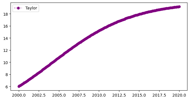
Results#
The plot below shows the 3rd order numerical approximation, \(w\) (circles) for the non-linear population equation:
fig = plt.figure(figsize=(8,4))
plt.plot(t,w,'o:',color='purple',label='Taylor')
plt.legend(loc='best')
plt.show()
Table#
The table below shows the time and the 3rd order numerical approximation, \(w\), for the non-linear population equation:
d = {'time t_i': t[0:10],    'Taylor ':w[0:10]}
df = pd.DataFrame(data=d)
df
| time t_i | Taylor | |
|---|---|---|
| 0 | 2000.0 | 6.000000 |
| 1 | 2000.1 | 6.084335 |
| 2 | 2000.2 | 6.169332 |
| 3 | 2000.3 | 6.254983 |
| 4 | 2000.4 | 6.341279 |
| 5 | 2000.5 | 6.428207 |
| 6 | 2000.6 | 6.515760 |
| 7 | 2000.7 | 6.603924 |
| 8 | 2000.8 | 6.692689 |
| 9 | 2000.9 | 6.782043 |
3. Non-Linear Population Equation with an oscilation#
with the initial condition, $\(y(2000)=6.\)$
Specific 3rd Order Taylor for the Non-Linear Population Equation with an oscilation#
To write the specific 3rd Order Taylor difference equation for the intial value problem we need calculate the first derivative of $\(f(t,y)=0.2y-0.01y^2+\sin(2\pi t),\)$
def nonlin_oscfun(t,w):
    ftw=0.2*w-0.01*w*w+np.sin(2*np.math.pi*t)
    return ftw
with respect to \(t\) $\( f'(t,y)=0.2y'-0.02y'y+2\pi\cos(2\pi t)\)\( \)\(=(0.2-0.02y)\big(0.2y-0.01y^2+\sin(2\pi t)\big)+2\pi\cos(2\pi t) \)$
def nonlin_oscfun_d(t,w):
    ftw=0.2*nonlinfun(t,w)-0.02*nonlinfun(t,w)*w+2*np.math.pi*np.cos(2*np.math.pi*t)
    return ftw
and the second derivative with respect to \(t\) $\( f''(t,y)=-0.02y'(0.2y-0.01y^2+\sin(2\pi t))\)\( \)\(+(0.2-0.02y)\big(0.2y'-0.02y'y+2\pi\cos(2\pi t)\big)-(2\pi)^2\sin(2\pi t)\)\( \)\(=-0.02(0.2y-0.01y^2+2\pi\sin(2\pi t))^2\)\( \)\(+(0.2-0.02y)\big((0.2-0.02y)(0.2y-0.01y^2+\sin(2\pi t))+ 2\pi\cos(2\pi t) \big)-(2\pi)^2\sin(2\pi t) \)$
def nonlin_oscfun_dd(t,w):
    ftw=-0.02*nonlin_oscfun(t,w)*nonlin_oscfun(t,w)+(0.2-0.02*w)*((0.2-0.02*w)*nonlin_oscfun(t,w)+2*np.math.pi*np.cos(2*np.math.pi*t))#-2*np.math.pi*2*np.math.pi*np.sin(2*np.math.pi*t)
    return ftw
Non-Linear Population with oscilation 3rd Order Taylor Difference equation#
Substituting the derivatives of the non-linear population equation with oscilation into the 3rd order Taylor equation gives the difference equation $\( w_{i+1}= w_{i} + h\big[\big(0.2w_i-0.01w_i^2+\sin(2\pi t_i)\big)\)\( \)\(+\frac{h}{2}\big((0.2-0.02w_i)\big(0.2w_i-0.01w_i^2+\sin(2\pi t_i)\big)+2\pi\cos(2\pi t_i)\big)+\)\( \)\(\frac{h^2}{6}\big(-0.02(0.2w_i-0.01w_i^2+2\pi\sin(2\pi t_i))^2\)\( \)\(+(0.2-0.02w_i)\big((0.2-0.02w_i)[0.2w_i-0.01w_i^2+\sin(2\pi t_i)]\)\( \)\(+ 2\pi\cos(2\pi t_i) \big)-(2\pi)^2\sin(2\pi t_i) \big)\big], \)\( for \)i=0,…,199\(, where \)w_i\( is the numerical approximation of \)y\( at time \)t_i\(, with the initial condition \)\(w_0=6.\)$
w=np.zeros(N+1)
w[0]=6.0
for i in range (0,N):
    w[i+1]=w[i]+h*(nonlin_oscfun(t[i],w[i])+h/2*nonlin_oscfun_d(t[i],w[i])+h*h/6*nonlin_oscfun_dd(t[i],w[i]))
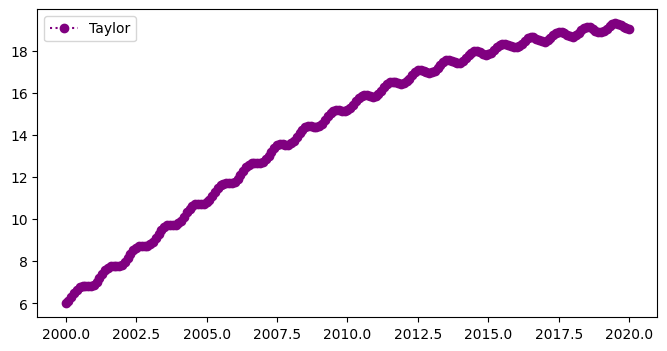
Results#
The plot below shows the 3rd order numerical approximation, \(w\) (circles) for the non-linear population equation:
fig = plt.figure(figsize=(8,4))
plt.plot(t,w,'o:',color='purple',label='Taylor')
plt.legend(loc='best')
plt.show()
Table#
The table below shows the time and the 3rd order numerical approximation, \(w\), for the non-linear population equation:
d = {'time t_i': t[0:10],    'Taylor ':w[0:10]}
df = pd.DataFrame(data=d)
df
| time t_i | Taylor | |
|---|---|---|
| 0 | 2000.0 | 6.000000 |
| 1 | 2000.1 | 6.115834 |
| 2 | 2000.2 | 6.285332 |
| 3 | 2000.3 | 6.476682 |
| 4 | 2000.4 | 6.649942 |
| 5 | 2000.5 | 6.772316 |
| 6 | 2000.6 | 6.830702 |
| 7 | 2000.7 | 6.836694 |
| 8 | 2000.8 | 6.822138 |
| 9 | 2000.9 | 6.826948 |