The Implicit Crank-Nicolson Difference Equation for the Heat Equation

The Heat Equation

The Heat Equation is the first order in time (\(t\)) and second order in space (\(x\)) Partial Differential Equation:

(632)\[\begin{equation} \frac{\partial u}{\partial t} = \frac{\partial^2 u}{\partial x^2},\end{equation}\]

The equation describes heat transfer on a domain

(633)\[\begin{equation}\Omega = \{ t \geq, 0\leq x \leq 1\}. \end{equation}\]

with an initial condition at time \(t=0\) for all \(x\) and boundary condition on the left (\(x=0\)) and right side (\(x=1\)).

Crank-Nicolson Difference method

This note book will illustrate the Crank-Nicolson Difference method for the Heat Equation with the initial conditions

(634)\[\begin{equation} u(x,0)=x^2, \ \ 0 \leq x \leq 1, \end{equation}\]

and boundary condition

(635)\[\begin{equation} u(0,t)=t, u(1,t)=2-exp(-t). \end{equation}\]

# LIBRARY
# vector manipulation
import numpy as np
# math functions
import math 

# THIS IS FOR PLOTTING
%matplotlib inline
import matplotlib.pyplot as plt # side-stepping mpl backend
import warnings
warnings.filterwarnings("ignore")

Discete Grid

The region \(\Omega\) is discretised into a uniform mesh \(\Omega_h\). In the space \(x\) direction into \(N\) steps giving a stepsize of

(636)\[\begin{equation} h=\frac{1-0}{N},\end{equation}\]

resulting in

(637)\[\begin{equation}x[i]=0+ih,\end{equation}\]

and into \(N_t\) steps in the time \(t\) direction giving a stepsize of

(638)\[\begin{equation}k=\frac{1-0}{N}\end{equation}\]

resulting in

(639)\[\begin{equation}t[i]=0+ik.\end{equation}\]

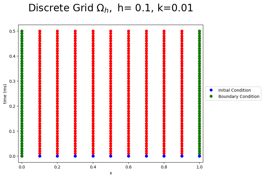
The Figure below shows the discrete grid points for \(N=10\) and \(N_t=15\), the red dots are the unknown values, the green dots are the known boundary conditions and the blue dots are the known initial conditions of the Heat Equation.

N=10
Nt=100
h=1/N
k=1/Nt
r=k/(h*h)
time_steps=50
time=np.arange(0,(time_steps+.5)*k,k)
x=np.arange(0,1.0001,h)
X, Y = np.meshgrid(x, time)
fig = plt.figure(figsize=(8,6))
plt.plot(X,Y,'ro');
plt.plot(x,0*x,'bo',label='Initial Condition');
plt.plot(np.ones(time_steps+1),time,'go',label='Boundary Condition');
plt.plot(x,0*x,'bo');
plt.plot(0*time,time,'go');
plt.xlim((-0.02,1.02))
plt.xlabel('x')
plt.ylabel('time (ms)')
plt.legend(loc='center left', bbox_to_anchor=(1, 0.5))
plt.title(r'Discrete Grid $\Omega_h,$ h= %s, k=%s'%(h,k),fontsize=24,y=1.08)
plt.show();

Discrete Initial and Boundary Conditions

The discrete initial conditions are

(640)\[\begin{equation}w[i,0]=x[i]\times x[i], \ \ 0 \leq x[i] \leq 1\end{equation}\]

and the discrete boundary conditions are

(641)\[\begin{equation}w[0,j]=t[j], w[10,j]=2-math.exp(t[j]), \end{equation}\]

where \(w[i,j]\) is the numerical approximation of \(U(x[i],t[j])\).

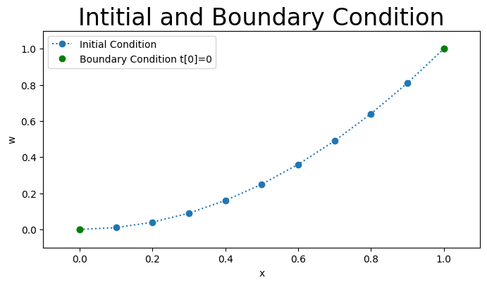
The Figure below plots the inital and boundary conditions for \(t[0]=0.\)

w=np.zeros((N+1,time_steps+1))
b=np.zeros(N-1)
# Initial Condition
for i in range (1,N):
    w[i,0]=x[i]*x[i]
    

# Boundary Condition
for j in range (0,time_steps+1):
    w[0,j]=time[j]
    w[N,j]=2-math.exp(-time[j])

fig = plt.figure(figsize=(8,4))
plt.plot(x,w[:,0],'o:',label='Initial Condition')
plt.plot(x[[0,N]],w[[0,N],0],'go',label='Boundary Condition t[0]=0')
plt.xlim([-0.1,1.1])
plt.ylim([-0.1,1.1])
plt.title('Intitial and Boundary Condition',fontsize=24)
plt.xlabel('x')
plt.ylabel('w')
plt.legend(loc='best')
plt.show()

The Implicit Crank-Nicolson Difference Equation

The implicit Crank-Nicolson difference equation of the Heat Equation is

(642)\[\begin{equation} \frac{w_{ij+1}-w_{ij}}{k}=\frac{1}{2}\left(\frac{w_{i+1j+1}-2w_{ij+1}+w_{i-1j+1}}{h^2}+\frac{w_{i+1j}-2w_{ij}+w_{i-1j}}{h^2}\right) \end{equation}\]

rearranging the equation we get

(643)\[\begin{equation} -rw_{i-1j+1}+(2+2r)w_{ij+1}-rw_{i+1j+1}=rw_{i-1j}+(2-2r)w_{ij}+rw_{i+1j} \end{equation}\]

for \(i=1,...9\) where \(r=\frac{k}{h^2}\).

This gives the formula for the unknown term \(w_{ij+1}\) at the \((ij+1)\) mesh points in terms of \(x[i]\) along the jth time row.

Hence we can calculate the unknown pivotal values of \(w\) along the first row of \(j=1\) in terms of the known boundary conditions.

This can be written in matrix form

(644)\[\begin{equation} A\mathbf{w}_{j+1}=B\mathbf{w}_{j} +\mathbf{b}_{j}+\mathbf{b}_{j+1} \end{equation}\]

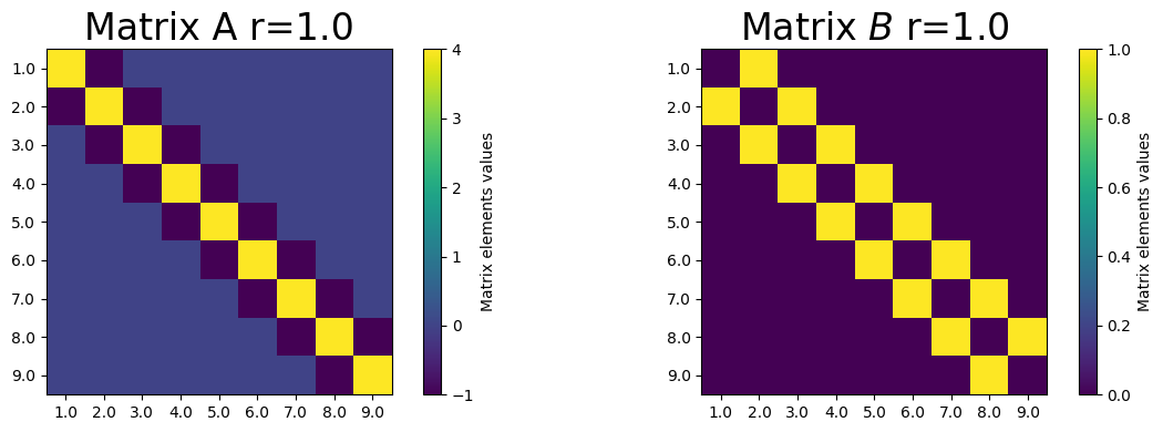
for which \(A\) is a \(9\times9\) matrix:

(645)\[\begin{equation} \left(\begin{array}{cccc cccc} 2+2r&-r& 0&0&0 &0&0&0\\ -r&2+2r&-r&0&0&0 &0&0&0\\ 0&-r&2+2r &-r&0&0& 0&0&0\\ 0&0&-r&2+2r &-r&0&0& 0&0\\ 0&0&0&-r&2+2r &-r&0&0& 0\\ 0&0&0&0&-r&2+2r &-r&0&0\\ 0&0&0&0&0&-r&2+2r &-r&0\\ 0&0&0&0&0&0&-r&2+2r&-r\\ 0&0&0&0&0&0&0&-r&2+2r\\ \end{array}\right) \left(\begin{array}{c} w_{1j+1}\\ w_{2j+1}\\ w_{3j+1}\\ w_{4j+1}\\ w_{5j+1}\\ w_{6j+1}\\ w_{7j+1}\\ w_{8j+1}\\ w_{9j+1}\\ \end{array}\right)= \left(\begin{array}{cccc cccc} 2-2r&r& 0&0&0 &0&0&0\\ r&2-2r&r&0&0&0 &0&0&0\\ 0&r&2-2r &r&0&0& 0&0&0\\ 0&0&r&2-2r &r&0&0& 0&0\\ 0&0&0&r&2-2r &r&0&0& 0\\ 0&0&0&0&r&2-2r &r&0&0\\ 0&0&0&0&0&r&2-2r &r&0\\ 0&0&0&0&0&0&r&2-2r&r\\ 0&0&0&0&0&0&0&r&2-2r\\ \end{array}\right) \left(\begin{array}{c} w_{1j}\\ w_{2j}\\ w_{3j}\\ w_{4j}\\ w_{5j}\\ w_{6j}\\ w_{7j}\\ w_{8j}\\ w_{9j}\\ \end{array}\right)+ \left(\begin{array}{c} rw_{0j}\\ 0\\ 0\\ 0\\ 0\\ 0\\ 0\\ 0\\ rw_{10j}\\ \end{array}\right)+ \left(\begin{array}{c} rw_{0j+1}\\ 0\\ 0\\ 0\\ 0\\ 0\\ 0\\ 0\\ rw_{10j+1}\\ \end{array}\right). \end{equation}\]

It is assumed that the boundary values \(w_{0j}\) and \(w_{10j}\) are known for \(j=1,2,...\), and \(w_{i0}\) for \(i=0,...,10\) is the initial condition.

The Figure below shows the matrix \(A\) and its inverse \(A^{-1}\) in color plot form for \(r\).

A=np.zeros((N-1,N-1))
B=np.zeros((N-1,N-1))
for i in range (0,N-1):
    A[i,i]=2+2*r
    B[i,i]=2-2*r

for i in range (0,N-2):           
    A[i+1,i]=-r
    A[i,i+1]=-r
    B[i+1,i]=r
    B[i,i+1]=r
    
Ainv=np.linalg.inv(A)   
fig = plt.figure(figsize=(12,4));
plt.subplot(121)
plt.imshow(A,interpolation='none');
plt.xticks(np.arange(N-1), np.arange(1,N-0.9,1));
plt.yticks(np.arange(N-1), np.arange(1,N-0.9,1));
clb=plt.colorbar();
clb.set_label('Matrix elements values');
plt.title('Matrix A r=%s'%(np.round(r,3)),fontsize=24)

plt.subplot(122)
plt.imshow(B,interpolation='none');
plt.xticks(np.arange(N-1), np.arange(1,N-0.9,1));
plt.yticks(np.arange(N-1), np.arange(1,N-0.9,1));
clb=plt.colorbar();
clb.set_label('Matrix elements values');
plt.title(r'Matrix $B$ r=%s'%(np.round(r,3)),fontsize=24)
fig.tight_layout()
plt.show();

Results

To numerically approximate the solution at \(t[1]\) the matrix equation becomes

(646)\[\begin{equation} \mathbf{w}_{1}=A^{-1}(B\mathbf{w}_{0} +\mathbf{b}_{1}+\mathbf{b}_{0})\end{equation}\]

where all the right hand side is known. To approximate solution at time \(t[2]\) we use the matrix equation

(647)\[\begin{equation} \mathbf{w}_{2}=A^{-1}(B\mathbf{w}_{1}+\mathbf{b}_{2} +\mathbf{b}_{1}). \end{equation}\]

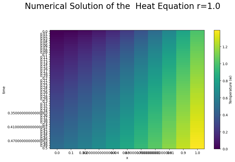
Each set of numerical solutions \(w[i,j]\) for all \(i\) at the previous time step is used to approximate the solution \(w[i,j+1]\). The left and right plot below show the numerical approximation \(w[i,j]\) of the Heat Equation using the BTCS method for \(x[i]\) for \(i=0,...,10\) and time steps \(t[j]\) for \(j=1,...,15\).

for j in range (1,time_steps+1):
    b[0]=r*w[0,j-1]+r*w[0,j]
    b[N-2]=r*w[N,j-1]+r*w[N,j]
    v=np.dot(B,w[1:(N),j-1])
    w[1:(N),j]=np.dot(Ainv,v+b)

fig = plt.figure(figsize=(10,6));
plt.imshow(w.transpose(), aspect='auto')
plt.xticks(np.arange(len(x)), x)
plt.yticks(np.arange(len(time)), time)
plt.xlabel('x')
plt.ylabel('time')
clb=plt.colorbar()
clb.set_label('Temperature (w)')
plt.suptitle('Numerical Solution of the  Heat Equation r=%s'%(np.round(r,3)),fontsize=24,y=1.08)
fig.tight_layout()
plt.show()