1 Step Adams Moulton

1 Step Adams Moulton#

John S Butler#

john.s.butler@tudublin.ie
Course Notes Github

This notebook implements the 1 step Adams Moulton method for three different population intial value problems.

Formula#

The general 1 step Adams-Moulton method for the first order differential equation

(247)#\[\begin{equation} y^{'} = f(t,y) \end{equation}\]

numerical approximates \(y\) the at time point \(t_i\) as \(w_i\) with the formula:

(248)#\[\begin{equation} w_{i+1}=w_i+\frac{h}{2}\big[f(t_{i+1},w_{i+1})+f(t_{i},w_{i})\big],\end{equation}\]

for \(i=0,...,N-1\), where

and \(h\) is the stepsize.

To illustrate the method we will apply it to three intial value problems:

1. Linear#

Consider the linear population Differential Equation

(249)#\[\begin{equation} y^{'}=0.1y, \ \ (2000 \leq t \leq 2020), \end{equation}\]

with the initial condition,

(250)#\[\begin{equation}y(2000)=6.\end{equation}\]

2. Non-Linear Population Equation#

Consider the non-linear population Differential Equation

(251)#\[\begin{equation} y^{'}=0.2y-0.01y^2, \ \ (2000 \leq t \leq 2020), \end{equation}\]

with the initial condition,

(252)#\[\begin{equation}y(2000)=6.\end{equation}\]

3. Non-Linear Population Equation with an oscillation#

Consider the non-linear population Differential Equation with an oscillation

(253)#\[\begin{equation} y^{'}=0.2y-0.01y^2+\sin(2\pi t), \ \ (2000 \leq t \leq 2020), \end{equation}\]

with the initial condition,

(254)#\[\begin{equation}y(2000)=6.\end{equation}\]

Setting up Libraries#

## Library
import numpy as np
import math 
import pandas as pd
%matplotlib inline
import matplotlib.pyplot as plt # side-stepping mpl backend
import matplotlib.gridspec as gridspec # subplots
import warnings

warnings.filterwarnings("ignore")

Discrete Interval#

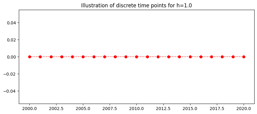
The continuous time \(a\leq t \leq b \) is discretised into \(N\) points seperated by a constant stepsize

(255)#\[\begin{equation} h=\frac{b-a}{N}.\end{equation}\]

Here the interval is \(2000\leq t \leq 2020,\)

(256)#\[\begin{equation} h=\frac{2020-2000}{200}=0.1.\end{equation}\]

This gives the 201 discrete points:

(257)#\[\begin{equation} t_0=2000, \ t_1=2000.1, \ ... t_{200}=2020. \end{equation}\]

This is generalised to

(258)#\[\begin{equation} t_i=2000+i0.1, \ \ \ i=0,1,...,200.\end{equation}\]

The plot below shows the discrete time steps:

### DISCRETE TIME
N=20
t_end=2020.0
t_start=2000.0
h=((t_end-t_start)/N)
t=np.arange(t_start,t_end+h/2,h)

## PLOTS TIME
fig = plt.figure(figsize=(10,4))
plt.plot(t,0*t,'o:',color='red')
plt.title('Illustration of discrete time points for h=%s'%(h))
plt.show()
len(t)

../_images/17c54b7d8b7b3ae02c8280ee2f692197d33894ae9803cc70f9127fde5c15d84c.png

1. Linear Population Equation#

Exact Solution#

The linear population equation

(259)#\[\begin{equation} y^{'}=0.1y, \ \ (2000 \leq t \leq 2020), \end{equation}\]

with the initial condition,

(260)#\[\begin{equation}y(2000)=6.\end{equation}\]

has a known exact (analytic) solution

(261)#\[\begin{equation} y(t)=6e^{0.1(t-2000)}. \end{equation}\]

Specific 1 step Adams Moulton#

The specific 1 step Adams Moulton for the linear population equation is:

(262)#\[\begin{equation}w_{i+1}=w_{i}+\frac{h}{2}\big[0.1w_{i+1}+0.1w_i\big] \end{equation}\]

where

(263)#\[\begin{equation}f(t,y)=0.1y,\end{equation}\]

## THIS IS THE RIGHT HANDSIDE OF THE LINEAR POPULATION DIFFERENTIAL 
## EQUATION
def linfun(t,w):
    ftw=0.1*w
    return ftw

re-arranging,

(264)#\[\begin{equation} \big(1-\frac{h}{2}(0.1)\big)w_{i+1}=w_i+\frac{h}{2}\big[0.1w_i\big], \end{equation}\]

(265)#\[\begin{equation} w_{i+1}=\frac{w_i+\frac{h}{2}\big[0.1w_i\big]}{\big(1-\frac{h}{2}(0.1)\big)}. \end{equation}\]

### INSERT METHOD HERE
w=np.zeros(N+1) # a list of 2000+1 zeros
w[0]=6 # INITIAL CONDITION
for i in range(0,N):
    w[i+1]=(w[i]+h/2*(linfun(t[i],w[i])))/(1-0.1*h/2)

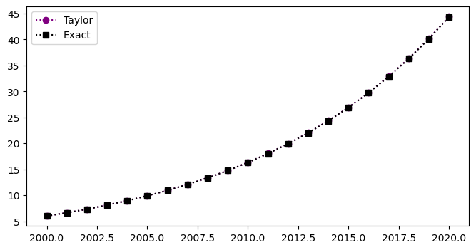
Plotting Results#

## PLOTTING METHOD
y=6*np.exp(0.1*(t-2000)) # EXACT SOLUTION
fig = plt.figure(figsize=(8,4))
plt.plot(t,w,'o:',color='purple',label='Taylor')
plt.plot(t,y,'s:',color='black',label='Exact')
plt.legend(loc='best')
plt.show()

../_images/56bee6b50cb6bf8ed5f8503879d4c94579e3e03e04a1303b3ce8b601072f9234.png

Table#

The table below shows the time, the numerical approximation, \(w\), the exact solution, \(y\), and the exact error \(|y(t_i)-w_i|\) for the linear population equation:

d = {'time t_i': t, 'Adams Approx w': w}
df = pd.DataFrame(data=d)
df

	time t_i	Adams Approx w
0	2000.0	6.000000
1	2001.0	6.631579
2	2002.0	7.329640
3	2003.0	8.101181
4	2004.0	8.953937
5	2005.0	9.896456
6	2006.0	10.938189
7	2007.0	12.089577
8	2008.0	13.362164
9	2009.0	14.768708
10	2010.0	16.323308
11	2011.0	18.041551
12	2012.0	19.940662
13	2013.0	22.039679
14	2014.0	24.359645
15	2015.0	26.923819
16	2016.0	29.757905
17	2017.0	32.890316
18	2018.0	36.352454
19	2019.0	40.179029
20	2020.0	44.408400

2. Non-Linear Population Equation#

(266)#\[\begin{equation} y^{'}=0.2y-0.01y^2, \ \ (2000 \leq t \leq 2020), \end{equation}\]

with the initial condition,

(267)#\[\begin{equation}y(2000)=6.\end{equation}\]

Specific 1 step Adams-Moutlon method for the Non-Linear Population Equation#

The specific Adams-Moulton difference equation for the non-linear population equations is:

(268)#\[\begin{equation}w_{i+1}=w_{i}+\frac{h}{2}\big[ 0.2 w_{i+1}-0.01 w_{i+1}^2 + 0.2 w_i-0.01 w_i^2\big] \end{equation}\]

re-arranging

(269)#\[\begin{equation}w_{i+1}-\frac{h}{2}\big( 0.2 w_{i+1}-0.01 w_{i+1}^2 \big)=w_{i}+\frac{h}{2} \big[ 0.2 w_i-0.01 w_i^2\big] \end{equation}\]

for \(i=0,...,199\), where \(w_i\) is the numerical approximation of \(y\) at time \(t_i\), with step size \(h\) and the initial condition

(270)#\[\begin{equation}w_0=6.\end{equation}\]

PROBLEM WE CANNOT MOVE THE SQUARED (NON-LINEAR TERM) TO THE RIGHT HAND SIDE SO WE CAN SOLVE FOR w[i+1]. For this reason we will use a predictor-corrector method, The predictor will be the 2-step Adams Bashforth

(271)#\[\begin{equation} w_{i+1}^{p}=w_{i}+\frac{h}{2}\big[ 3(0.2 w_{i}-0.01 w_{i}^2) - (0.2 w_{i-1}-0.01 w_{i-1}^2) \big], \end{equation}\]

with the corrector being the 1-step Adams Moulton,

(272)#\[\begin{equation}w_{i+1}=w_{i}+\frac{h}{2}\big[ 0.2 w_{i+1}^p-0.01 (w^p_{i+1})^2 + 0.2 w_i-0.01 w_i^2\big], \end{equation}\]

for i=1,…200.

def nonlinfun(t,w):
    ftw=0.2*w-0.01*w*w
    return ftw

### INSERT METHOD HERE
w=np.zeros(N+1)
w_p=np.zeros(N+1)
w[0]=6
w[1]=6.084 # FROM THE THE TAYLOR METHOD
w_p[0]=6
w_p[1]=6.084 # FROM THE THE TAYLOR METHOD
for n in range(1,N):
    ## Predictor
    w_p[n+1]=w[n]+h/2*(3*nonlinfun(t[n],w[n])-
                       nonlinfun(t[n-1],w[n-1]))
    ## Corrector
    w[n+1]=w[n]+h/2*(nonlinfun(t[n+1],w_p[n+1])+
                       nonlinfun(t[n],w[n]))

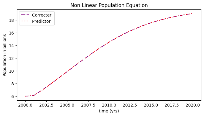
Results#

The plot below shows the numerical approximation, \(w\) (circles) for the non-linear population equation:

fig = plt.figure(figsize=(8,4))
plt.plot(t,w,'-.',color='purple',label='Correcter ')
plt.plot(t,w_p,':',color='red',label='Predictor ')

plt.title('Non Linear Population Equation')
plt.legend(loc='best')
plt.xlabel('time (yrs)')
plt.ylabel('Population in billions')
plt.show()

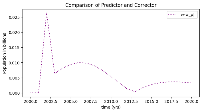
fig = plt.figure(figsize=(8,4))
plt.plot(t,np.abs(w-w_p),':',color='purple',label='|w-w_p| ')
plt.title('Comparison of Predictor and Corrector')
plt.legend(loc='best')
plt.xlabel('time (yrs)')
plt.ylabel('Population in billions')
plt.show()

../_images/d56d9d2640e44fbc27eff704dc849d3a693bc7588ff04a2bc2d026403781c4f2.png

../_images/90686d0fb616a5d80a03526cb557f432e99d810c476836c5efef13d2f00afd99.png

Table#

The table below shows the time and the numerical approximation, \(w\), for the non-linear population equation:

d = {'time t_i': t, 'Adams Approx w': w}
df = pd.DataFrame(data=d)
df

	time t_i	Adams Approx w
0	2000.0	6.000000
1	2001.0	6.084000
2	2002.0	6.960322
3	2003.0	7.892040
4	2004.0	8.863456
5	2005.0	9.856908
6	2006.0	10.853082
7	2007.0	11.832473
8	2008.0	12.776881
9	2009.0	13.670688
10	2010.0	14.501747
11	2011.0	15.261810
12	2012.0	15.946493
13	2013.0	16.554881
14	2014.0	17.088907
15	2015.0	17.552635
16	2016.0	17.951549
17	2017.0	18.291930
18	2018.0	18.580348
19	2019.0	18.823293
20	2020.0	19.026909

3. Non-Linear Population Equation with an oscilation#

(273)#\[\begin{equation} y^{'}=0.2y-0.01y^2+\sin(2\pi t), \ \ (2000 \leq t \leq 2020), \end{equation}\]

with the initial condition,

(274)#\[\begin{equation}y(2000)=6.\end{equation}\]

Specific 2 Step Adams Moulton for the Non-Linear Population Equation with an oscilation#

The specific Adams-Moulton difference equation for the non-linear population equations is:

(275)#\[\begin{equation}w_{i+1}=w_{i}+\frac{h}{2}\big[ 0.2 w_{i+1}-0.01 w_{i+1}^2 +\sin(2\pi t_{i+1}) + 0.2 w_i-0.01 w_i^2+\sin(2\pi t_{i})\big] \end{equation}\]

for \(i=1,...,199\), where \(w_i\) is the numerical approximation of \(y\) at time \(t_i\), with step size \(h\) and the initial condition

(276)#\[\begin{equation}w_0=6.\end{equation}\]

As \(w_1\) is required for the method but unknown we will use the numerical solution of a one step method to approximate the value. Here, we use the 2nd order Runge Kutta approximation (see Runge Kutta notebook )

(277)#\[\begin{equation}w_1=6.11.\end{equation}\]

PROBLEM WE CANNOT MOVE THE SQUARED (NON-LINEAR TERM) TO THE RIGHT HAND SIDE SO WE CAN SOLVE FOR w[i+1]. For this reason we will use a predictor-corrector method, The predictor will be the 2-step Adams Bashforth

(278)#\[\begin{equation} w_{i+1}^{p}=w_{i}+\frac{h}{2}\big[ 3(0.2 w_{i}-0.01 w_{i}^2+\sin(2\pi t_{i}) - (0.2 w_{i-1}-0.01 w_{i-1}^2+\sin(2\pi t_{i-1}) \big] \end{equation}\]

with the corrector being the 1-step Adams Moulton,

(279)#\[\begin{equation}w_{i+1}=w_{i}+\frac{h}{2}\big[ 0.2 w_{i+1}^p-0.01 (w^p_{i+1})^2 +\sin(2\pi t_{i+1} + 0.2 w_i-0.01 w_i^2+\sin(2\pi t_{i}\big], \end{equation}\]

def nonlin_oscfun(t,w):
    ftw=0.2*w-0.01*w*w+np.sin(2*np.math.pi*t)
    return ftw

## INSERT METHOD HERE
w=np.zeros(N+1)
w[0]=6
w[1]=6.11
for n in range(1,N):
    w[n+1]=w[n]+h/2

Results#

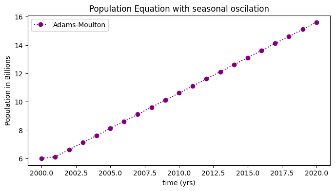
The plot below shows the numerical approximation, \(w\) (circles) for the non-linear population equation:

fig = plt.figure(figsize=(8,4))
plt.plot(t,w,'o:',color='purple',label='Adams-Moulton')
plt.title('Population Equation with seasonal oscilation')
plt.xlabel('time (yrs)')
plt.ylabel('Population in Billions')
plt.legend(loc='best')
plt.show()

../_images/2e3ba84c89215cf7d4d9c84034826415e3aa97c41a1809c96ce1defd831f70df.png

Table#

The table below shows the time and the numerical approximation, \(w\), for the non-linear population equation:

d = {'time t_i': t, 'Adams Approx w': w}
df = pd.DataFrame(data=d)
df

	time t_i	Adams Approx w
0	2000.0	6.00
1	2001.0	6.11
2	2002.0	6.61
3	2003.0	7.11
4	2004.0	7.61
5	2005.0	8.11
6	2006.0	8.61
7	2007.0	9.11
8	2008.0	9.61
9	2009.0	10.11
10	2010.0	10.61
11	2011.0	11.11
12	2012.0	11.61
13	2013.0	12.11
14	2014.0	12.61
15	2015.0	13.11
16	2016.0	13.61
17	2017.0	14.11
18	2018.0	14.61
19	2019.0	15.11
20	2020.0	15.61

1 Step Adams Moulton

Contents

1 Step Adams Moulton#

John S Butler#

Formula#

1. Linear#

2. Non-Linear Population Equation#

3. Non-Linear Population Equation with an oscillation#

Setting up Libraries#

Discrete Interval#

1. Linear Population Equation#

Exact Solution#

Specific 1 step Adams Moulton#

Plotting Results#

Table#

2. Non-Linear Population Equation#

Specific 1 step Adams-Moutlon method for the Non-Linear Population Equation#

Results#

Table#

3. Non-Linear Population Equation with an oscilation#

Specific 2 Step Adams Moulton for the Non-Linear Population Equation with an oscilation#

Results#

Table#