2 Step Adam Bashforth

2 Step Adam Bashforth#

John S Butler#

john.s.butler@tudublin.ie
Course Notes Github

This notebook implements the 2 step Adams Bashforth method for three different population intial value problems.

Formula#

The general 2 step Adams-Bashforth method for the first order differential equation

(200)#\[\begin{equation} y^{'} = f(t,y), \end{equation}\]

numerical approximates \(y\) the at time point \(t_i\) as \(w_i\) with the formula:

(201)#\[\begin{equation} w_{i+1}=w_i+\frac{h}{2}\big[3f(t_i,w_i)-f(t_{i-1},w_{i-1})\big],\end{equation}\]

for \(i=0,...,N-1\), where

and \(h\) is the stepsize.

To illustrate the method we will apply it to three intial value problems:

1. Linear#

Consider the linear population Differential Equation

(202)#\[\begin{equation} y^{'}=0.1y, \ \ (2000 \leq t \leq 2020), \end{equation}\]

with the initial condition,

(203)#\[\begin{equation}y(2000)=6.\end{equation}\]

2. Non-Linear Population Equation#

Consider the non-linear population Differential Equation

(204)#\[\begin{equation} y^{'}=0.2y-0.01y^2, \ \ (2000 \leq t \leq 2020), \end{equation}\]

with the initial condition,

(205)#\[\begin{equation}y(2000)=6.\end{equation}\]

3. Non-Linear Population Equation with an oscillation#

Consider the non-linear population Differential Equation with an oscillation

(206)#\[\begin{equation} y^{'}=0.2y-0.01y^2+\sin(2\pi t), \ \ (2000 \leq t \leq 2020), \end{equation}\]

with the initial condition,

(207)#\[\begin{equation}y(2000)=6.\end{equation}\]

Setting up Libraries#

## Library
import numpy as np
import math 
import pandas as pd

%matplotlib inline
import matplotlib.pyplot as plt # side-stepping mpl backend
import matplotlib.gridspec as gridspec # subplots
import warnings

warnings.filterwarnings("ignore")

Discrete Interval#

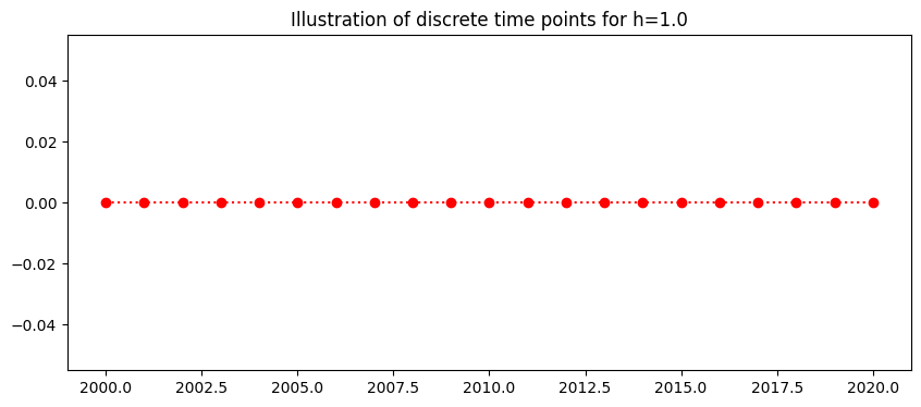
The continuous time \(a\leq t \leq b \) is discretised into \(N\) points seperated by a constant stepsize

(208)#\[\begin{equation} h=\frac{b-a}{N}.\end{equation}\]

Here the interval is \(2000\leq t \leq 2020,\)

(209)#\[\begin{equation} h=\frac{2020-2000}{200}=0.1.\end{equation}\]

This gives the 201 discrete points:

(210)#\[\begin{equation} t_0=2000, \ t_1=2000.1, \ ... t_{200}=2020. \end{equation}\]

This is generalised to

(211)#\[\begin{equation} t_i=2000+i0.1, \ \ \ i=0,1,...,200.\end{equation}\]

The plot below shows the discrete time steps:

### DISCRETE TIME
N=20
t_end=2020.0
t_start=2000.0
h=((t_end-t_start)/N)
t=np.arange(t_start,t_end+h/2,h)

## PLOTS TIME
fig = plt.figure(figsize=(10,4))
plt.plot(t,0*t,'o:',color='red')
plt.title('Illustration of discrete time points for h=%s'%(h))
plt.show()
len(t)

../_images/17c54b7d8b7b3ae02c8280ee2f692197d33894ae9803cc70f9127fde5c15d84c.png

1. Linear Population Equation#

Exact Solution#

The linear population equation

(212)#\[\begin{equation} y^{'}=0.1y, \ \ (2000 \leq t \leq 2020), \end{equation}\]

with the initial condition,

(213)#\[\begin{equation}y(2000)=6.\end{equation}\]

has a known exact (analytic) solution

(214)#\[\begin{equation} y(t)=6e^{0.1(t-2000)}. \end{equation}\]

Specific 2 step Adams Bashforth#

The specific 2 step Adams Bashforth for the linear population equation is:

(215)#\[\begin{equation}w_{i+1}=w_{i}+\frac{h}{2}\big[3(f(t_i,w_i))-f(t_{i-1},w_{i-1}))\big] \end{equation}\]

where

(216)#\[\begin{equation}f(t,y)=0.1y.\end{equation}\]

## THIS IS THE RIGHT HANDSIDE OF THE LINEAR POPULATION DIFFERENTIAL 
## EQUATION
def linfun(t,w):
    ftw=0.1*w
    return ftw

this gives

(217)#\[\begin{equation} w_{i+1}=w_{i}+\frac{0.1}{2}\big[ 3(0.1w_i)-0.1w_{i-1} \big]\end{equation}\]

for \(i=1,...,199\), where \(w_i\) is the numerical approximation of \(y\) at time \(t_i\), with step size \(h\) and the initial condition

(218)#\[\begin{equation}w_0=6.\end{equation}\]

### INSERT METHOD HERE
w=np.zeros(N+1) # a list of 2000+1 zeros
w[0]=6 # INITIAL CONDITION
w[1]=6.06
for i in range(1,N):
    w[i+1]=w[i]+h/2*(3*linfun(t[i],w[i])-linfun(t[i-1],w[i-1]))

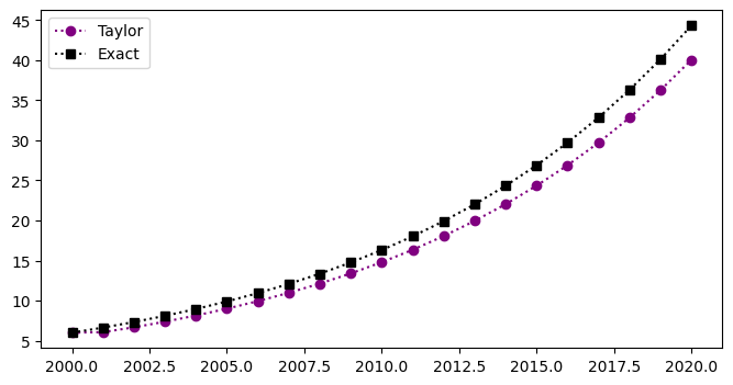
Plotting Results#

## PLOTTING METHOD
y=6*np.exp(0.1*(t-2000)) # EXACT SOLUTION
fig = plt.figure(figsize=(8,4))
plt.plot(t,w,'o:',color='purple',label='Taylor')
plt.plot(t,y,'s:',color='black',label='Exact')
plt.legend(loc='best')
plt.show()

../_images/82fccbd7c447ac2ec00591b3a8243843c79782b2b678ce9cdb0436dc8d774e47.png

Table#

The table below shows the time, the numerical approximation, \(w\), the exact solution, \(y\), and the exact error \(|y(t_i)-w_i|\) for the linear population equation:

d = {'time t_i': t, 'Adams w': w,'Exact y(t_i)':y,'Exact Error |w_i-y_i|':np.abs(y-w)}
df = pd.DataFrame(data=d)
df

	time t_i	Adams w	Exact y(t_i)	Exact Error \|w_i-y_i\|
0	2000.0	6.000000	6.000000	0.000000
1	2001.0	6.060000	6.631026	0.571026
2	2002.0	6.669000	7.328417	0.659417
3	2003.0	7.366350	8.099153	0.732803
4	2004.0	8.137852	8.950948	0.813096
5	2005.0	8.990213	9.892328	0.902115
6	2006.0	9.931852	10.932713	1.000861
7	2007.0	10.972119	12.082516	1.110397
8	2008.0	12.121345	13.353246	1.231901
9	2009.0	13.390940	14.757619	1.366678
10	2010.0	14.793514	16.309691	1.516177
11	2011.0	16.342994	18.024996	1.682002
12	2012.0	18.054768	19.920702	1.865934
13	2013.0	19.945833	22.015780	2.069947
14	2014.0	22.034970	24.331200	2.296230
15	2015.0	24.342924	26.890134	2.547211
16	2016.0	26.892614	29.718195	2.825581
17	2017.0	29.709360	32.843684	3.134325
18	2018.0	32.821133	36.297885	3.476752
19	2019.0	36.258835	40.115367	3.856532
20	2020.0	40.056603	44.334337	4.277733

2. Non-Linear Population Equation#

(219)#\[\begin{equation} y^{'}=0.2y-0.01y^2, \ \ (2000 \leq t \leq 2020), \end{equation}\]

with the initial condition,

(220)#\[\begin{equation}y(2000)=6.\end{equation}\]

Specific 2 step Adams-Bashforth method for the Non-Linear Population Equation#

The specific Adams-Bashforth difference equation for the non-linear population equations is:

(221)#\[\begin{equation}w_{i+1}=w_{i}+\frac{0.1}{2}\big[3(0.2w_{i}-0.01w_{i}^2)- (0.2w_{i-1}-0.01w_{i-1}^2)\big], \end{equation}\]

for \(i=1,...,199\), where \(w_i\) is the numerical approximation of \(y\) at time \(t_i\), with step size \(h\) and the initial condition

(222)#\[\begin{equation}w_0=6.\end{equation}\]

To solve the 2 step method we need a value for \(w_1\), here, we will use the approximation from the 2nd order Taylor method (see other notebook),

(223)#\[\begin{equation}w_1=6.084.\end{equation}\]

def nonlinfun(t,w):
    ftw=0.2*w-0.01*w*w
    return ftw

### INSERT METHOD HERE
w=np.zeros(N+1)
w[0]=6
w[1]=6.084 # FROM THE THE TAYLOR METHOD
for n in range(1,N):
    w[n+1]=w[n]+h/2*(3*nonlinfun(t[n],w[n])-nonlinfun(t[n-1],w[n-1]))

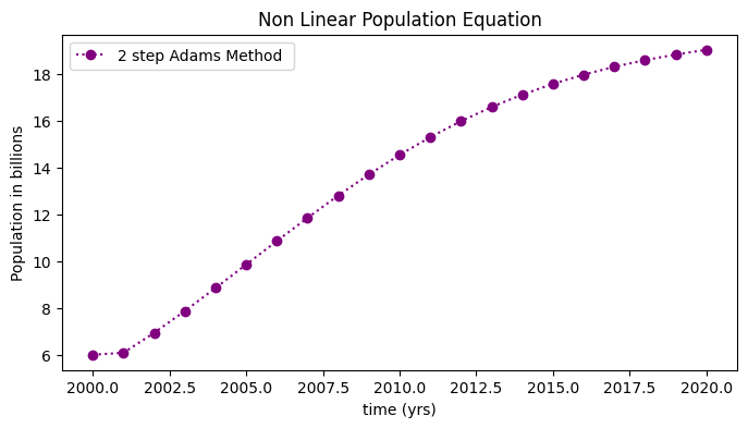
Results#

The plot below shows the numerical approximation, \(w\) (circles) for the non-linear population equation:

fig = plt.figure(figsize=(8,4))
plt.plot(t,w,'o:',color='purple',label='2 step Adams Method ')
plt.title('Non Linear Population Equation')
plt.legend(loc='best')
plt.xlabel('time (yrs)')
plt.ylabel('Population in billions')
plt.show()

../_images/557e626b19cb4ace0cbac1e5ececfb8702f928db06c78679d998931c28a05e50.png

Table#

The table below shows the time and the numerical approximation, \(w\), for the non-linear population equation:

d = {'time t_i': t, 'Adams approx of non-linear w': w}
df = pd.DataFrame(data=d)
df

	time t_i	Adams approx of non-linear w
0	2000.0	6.000000
1	2001.0	6.084000
2	2002.0	6.933974
3	2003.0	7.869642
4	2004.0	8.848568
5	2005.0	9.851373
6	2006.0	10.857671
7	2007.0	11.846747
8	2008.0	12.799268
9	2009.0	13.698782
10	2010.0	14.532747
11	2011.0	15.292965
12	2012.0	15.975461
13	2013.0	16.579947
14	2014.0	17.109042
15	2015.0	17.567443
16	2016.0	17.961143
17	2017.0	18.296777
18	2018.0	18.581128
19	2019.0	18.820774
20	2020.0	19.021862

3. Non-Linear Population Equation with an oscilation#

(224)#\[\begin{equation} y^{'}=0.2y-0.01y^2+\sin(2\pi t), \ \ (2000 \leq t \leq 2020), \end{equation}\]

with the initial condition,

(225)#\[\begin{equation}y(2000)=6.\end{equation}\]

Specific 2 Step Adams Bashforth for the Non-Linear Population Equation with an oscilation#

To write the specific

(226)#\[\begin{equation} w_{i+1}=w_{i}+\frac{0.1}{2} \big[ 3(0.2w_{i}-0.01w_{i}^2+\sin(2\pi t_{i}))- (0.2w_{i-1}-0.01w_{i-1}^2+\sin(2\pi t_{i-1}))\big] \end{equation}\]

for \(i=1,...,199\), where \(w_i\) is the numerical approximation of \(y\) at time \(t_i\), with step size \(h\) and the initial condition

(227)#\[\begin{equation}w_0=6.\end{equation}\]

As \(w_1\) is required for the method but unknown we will use the numerical solution of a one step method to approximate the value. Here, we use the 2nd order Runge Kutta approximation (see Runge Kutta notebook )

(228)#\[\begin{equation}w_1=6.11.\end{equation}\]

def nonlin_oscfun(t,w):
    ftw=0.2*w-0.01*w*w+np.sin(2*np.math.pi*t)
    return ftw

## INSERT METHOD HERE
w=np.zeros(N+1)
w[0]=6
w[1]=6.11
for n in range(1,N):
    w[n+1]=w[n]+h/2*(3*nonlin_oscfun(t[n],w[n])
                     -nonlin_oscfun(t[n-1],w[n-1]))

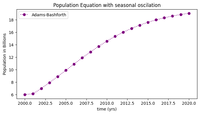
Results#

The plot below shows the numerical approximation, \(w\) (circles) for the non-linear population equation:

fig = plt.figure(figsize=(8,4))
plt.plot(t,w,'o:',color='purple',label='Adams-Bashforth')
plt.title('Population Equation with seasonal oscilation')
plt.xlabel('time (yrs)')
plt.ylabel('Population in Billions')
plt.legend(loc='best')
plt.show()

../_images/ac73546ffa6edec1ff2efa4195364af6cff8847894da72cc72033a76dde410ea.png

Table#

The table below shows the time and the numerical approximation, \(w\), for the non-linear population equation with oscilations:

d = {'time t_i': t, 'Adams Approx w': w}
df = pd.DataFrame(data=d)
df

	time t_i	Adams Approx w
0	2000.0	6.000000
1	2001.0	6.110000
2	2002.0	6.963018
3	2003.0	7.900330
4	2004.0	8.880317
5	2005.0	9.883555
6	2006.0	10.889620
7	2007.0	11.877816
8	2008.0	12.828881
9	2009.0	13.726473
10	2010.0	14.558187
11	2011.0	15.315964
12	2012.0	15.995957
13	2013.0	16.597982
14	2014.0	17.124739
15	2015.0	17.580977
16	2016.0	17.972719
17	2017.0	18.306611
18	2018.0	18.589435
19	2019.0	18.827758
20	2020.0	19.027711

2 Step Adam Bashforth

Contents

2 Step Adam Bashforth#

John S Butler#

Formula#

1. Linear#

2. Non-Linear Population Equation#

3. Non-Linear Population Equation with an oscillation#

Setting up Libraries#

Discrete Interval#

1. Linear Population Equation#

Exact Solution#

Specific 2 step Adams Bashforth#

Plotting Results#

Table#

2. Non-Linear Population Equation#

Specific 2 step Adams-Bashforth method for the Non-Linear Population Equation#

Results#

Table#

3. Non-Linear Population Equation with an oscilation#

Specific 2 Step Adams Bashforth for the Non-Linear Population Equation with an oscilation#

Results#

Table#