1st vs 2nd order Taylor methods

Intial Value Poblem

The general form of the population growth differential equation

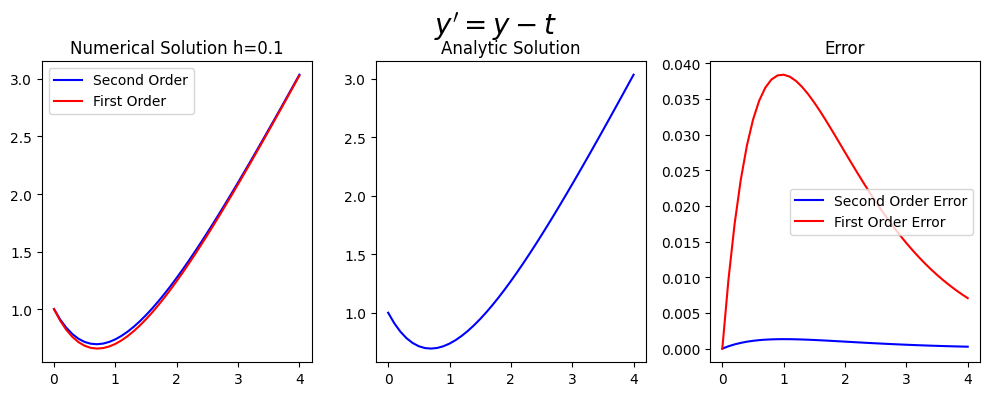
(105)\[\begin{equation} y^{'}=t-y, \ \ (0 \leq t \leq 4), \end{equation}\]

with the initial condition

(106)\[\begin{equation}x(0)=1, \end{equation}\]

For N=4 with the analytic (exact) solution

(107)\[\begin{equation} y= 2e^{-t}+t+1. \end{equation}\]

Taylor Solution

(108)\[\begin{equation} f(t,y)=t-y, \end{equation}\]

differentiate with respect to \(t\),

(109)\[\begin{equation} f'(t,y)=1-y'=1-t+y, \end{equation}\]

This gives the first order Taylor,

(110)\[\begin{equation}T^1(t_i,w,i)=f(t_i,w_i)=t_i-w_i, \end{equation}\]

and the second order Taylor,

(111)\[\begin{equation} T^2(t_i,w,i)=f(t_i,w_i)+\frac{h}{2}f'(t_i,w_i)=t_i-w_i+\frac{h}{2}(1-t_i+w_i).\end{equation}\]

The first order Taylor difference equation, which is identical to the Euler method, is

(112)\[\begin{equation} w_{i+1}=w_i+h(t_i-w_i). \end{equation}\]

The second order Taylor difference equation is

(113)\[\begin{equation} w_{i+1}=w_i+h(t_i-w_i+\frac{h}{2}(1-t_i+w_i)). \end{equation}\]

import numpy as np
import math 

%matplotlib inline
import matplotlib.pyplot as plt # side-stepping mpl backend
import matplotlib.gridspec as gridspec # subplots
import warnings

warnings.filterwarnings("ignore")

def Second_order_taylor(N,IC):
    x_end=4
    x_start=0
    
    INTITIAL_CONDITION=IC
    h=x_end/(N)
    N=N+1;
    Numerical_Solution=np.zeros(N)
    Numerical_Solution_first=np.zeros(N)
    t=np.zeros(N)
    Analytic_Solution=np.zeros(N)
    Upper_bound=np.zeros(N)
    
    t[0]=x_start
    Numerical_Solution[0]=INTITIAL_CONDITION
    Numerical_Solution_first[0]=INTITIAL_CONDITION
    Analytic_Solution[0]=INTITIAL_CONDITION
    for i in range (1,N):
        Numerical_Solution_first[i]=Numerical_Solution_first[i-1]+h*(t[i-1]-Numerical_Solution_first[i-1])
        Numerical_Solution[i]=Numerical_Solution[i-1]+h*(t[i-1]-Numerical_Solution[i-1]+h/2*(1-t[i-1]+Numerical_Solution[i-1]))
        t[i]=t[i-1]+h
        Analytic_Solution[i]=2*math.exp(-t[i])+t[i]-1
    

    fig = plt.figure(figsize=(10,4))
    # --- left hand plot
    ax = fig.add_subplot(1,3,1)
    plt.plot(t,Numerical_Solution,color='blue',label='Second Order')
    plt.plot(t,Numerical_Solution_first,color='red',label='First Order')
    plt.legend(loc='best')
    plt.title('Numerical Solution h=%s'%(h))

    # --- right hand plot
    ax = fig.add_subplot(1,3,2)
    plt.plot(t,Analytic_Solution,color='blue')
    plt.title('Analytic Solution')

    #ax.legend(loc='best')
    ax = fig.add_subplot(1,3,3)
    plt.plot(t,np.abs(Analytic_Solution-Numerical_Solution),color='blue',label='Second Order Error')
    plt.plot(t,np.abs(Analytic_Solution-Numerical_Solution_first),color='red',label='First Order Error')
    plt.title('Error')
    plt.legend(loc='best')
    # --- title, explanatory text and save
    
   
    # --- title, explanatory text and save
    fig.suptitle(r"$y'=y-t$", fontsize=20)
    plt.tight_layout()
    plt.subplots_adjust(top=0.85)    

Second_order_taylor(40,1)