Convergence of a Multistep Method

Convergence of a Multistep Method#

John S Butler#

john.s.butler@tudublin.ie
Course Notes Github

Overview#

A one-step or multistep method is used to approximate the solution of an initial value problem of the form

(342)#\[\begin{equation} \frac{dy}{dt}=f(t,y),\end{equation}\]

with the initial condition

(343)#\[\begin{equation} y(a)=\alpha.\end{equation}\]

The method should only be used if it satisfies the three criteria:

that difference equation is consistent with the differential equation;
that the numerical solution convergent to the exact answer of the differential equation;
that the numerical solution is stable.

In the notebooks in this folder we will illustate examples of consistent and inconsistent, convergent and non-convergent, and stable and unstable methods.

Introduction to Convergence#

In this notebook we will illustate an non-convergent method. The video below outlines the notebook.

from IPython.display import HTML
HTML('<iframe width="560" height="315" src="https://www.youtube.com/embed/skJSvK52nq0" frameborder="0" allow="accelerometer; autoplay; clipboard-write; encrypted-media; gyroscope; picture-in-picture" allowfullscreen></iframe>')

/Users/johnbutler/opt/anaconda3/lib/python3.8/site-packages/IPython/core/display.py:724: UserWarning: Consider using IPython.display.IFrame instead
  warnings.warn("Consider using IPython.display.IFrame instead")

Definition#

The solution of a multi-step methods $w_i$ is said to be convergent with respect to the exact solution of the differential equation if

(344)#\[\begin{equation} \max_{h \rightarrow 0}\max_{1 \leq i \leq N}|y(t_i)-w_i|=0.\end{equation}\]

All the Runge Kutta, Adams-Bashforth and Adams-Moulton methods are convergent.

2-step Abysmal Butler Multistep Method#

This notebook will illustrate a non-convergent multistep method using the Abysmal-Butler method, named with great pride after the author. The 2-step Abysmal Butler difference equation is given by

(345)#\[\begin{equation}w_{i+1} = w_{i} + \frac{h}{2}(4f(t_i,w_i)-3f(t_{i-1},w_{i-1})),\end{equation}\]

The final section of this notebooks shows that the method is non-convergent for all differential equations.

Intial Value Problem#

To illustrate convergence we will apply Abysmal-Butler multistep method to the linear intial value problem

(346)#\[\begin{equation} y^{'}=t-y, \ \ (0 \leq t \leq 2) \end{equation}\]

with the initial condition

(347)#\[\begin{equation}y(0)=1,\end{equation}\]

with the exact solution

(348)#\[\begin{equation}y(t)= 2e^{-t}+t-1.\end{equation}\]

Python Libraries#

import numpy as np
import math 
import pandas as pd


%matplotlib inline
import matplotlib.pyplot as plt # side-stepping mpl backend
import matplotlib.gridspec as gridspec # subplots
import warnings

warnings.filterwarnings("ignore")

Defining the function#

(349)#\[\begin{equation}f(t,y)=t-y.\end{equation}\]

def myfun_ty(t,y):
    return t-y

Discrete Interval#

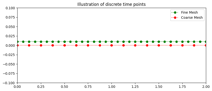
To illustrtate that the method is internally convergent but not convergent with the exact solution we define two discrete meshes, one coarse and one fine.

Coarse mesh#

Defining the step size $h$ from the interval range $a \leq t \leq b$ and number of steps $N$

(350)#\[\begin{equation}h=\frac{b - a}{N}.\end{equation}\]

This gives the discrete time steps, $$t_i=t_0+ih,$$ where $t_0=a,$ for $i=0,1…,N$.

Fine mesh#

Defining the step size $h/2$ from the interval range $a≤t≤b$ and number of steps $2N$

(351)#\[\begin{equation}h=\frac{b−a}{2N}.\end{equation}\]

This gives the discrete time steps,

(352)#\[\begin{equation}t_i=t_0+ih,\end{equation}\]

where $t_0=a,$ for $i =0,1,...2N$.

The plot below shows the coarse (red) and fine (green) discrete time intervals over the domain.

# Start and end of interval
b=2
a=0
# Step size
N=16
h=(b-a)/(N)
t=np.arange(a,b+h,h)
N2=N*2
h2=(b-a)/(N2)
t2=np.arange(a,b+h2,h2)
w2=np.zeros(len(t2))

fig = plt.figure(figsize=(10,4))
plt.plot(t2,0.01*np.ones(len(t2)),'o:',color='green',label='Fine Mesh')
plt.plot(t,0*t,'o:',color='red',label='Coarse Mesh')
plt.xlim((0,2))
plt.ylim((-0.1,.1))

plt.legend()
plt.title('Illustration of discrete time points')
plt.show()

../_images/cd78b945680f172b4e30d927384fb4d6c3531bb276c44271e8b8921694f3fb8a.png

2-step Abysmal Butler Method#

The 2-step Abysmal Butler difference equation is

(353)#\[\begin{equation}w_{i+1} = w_{i} + \frac{h}{2}(4(t_i-w_i)-3(t_{i-1}-w_{i-1})), \end{equation}\]

for $i=1,...N.$ For $i=0$ the system of difference equation is:

(354)#\[\begin{equation}w_{1} = w_{0} + \frac{h}{2}(4(t_0-w_0)-3(t_{-1}-w_{-1})) \end{equation}\]

this is not solvable as $w_{-1}$ is unknown.

For $i=1$ the difference equation is:

(355)#\[\begin{equation}w_{2} = w_{1} + \frac{h}{2}(4(t_1-w_1)-3(t_{0}-w_{0})) \end{equation}\]

this is not solvable a $w_{1}$ is unknown. $w_1$ can be approximated using a one step method. Here, as the exact solution is known,

(356)#\[\begin{equation}w_1=2e^{-t_1}+t_1-1.\end{equation}\]

### Initial conditions
IC=1
w=np.zeros(len(t))
w[0]=IC

w2=np.zeros(len(t2))
w2[0]=IC
w2[1]=(IC+1)*np.exp(-t2[1])+t2[1]-1

Loop#

# Fine Mesh
for k in range (1,N2):
    w2[k+1]=(w2[k]+h2/2.0*(4*myfun_ty(t2[k],w2[k])-3*myfun_ty(t2[k-1],w2[k-1]))) 
    
    
w[1]=w2[2]

# Coarse Mesh
for k in range (1,N):
    w[k+1]=(w[k]+h/2.0*(4*myfun_ty(t[k],w[k])-3*myfun_ty(t[k-1],w[k-1])))   

Plotting solution#

def plotting(t,w,t2,w2):
    y=(2)*np.exp(-t2)+t2-1
    fig = plt.figure(figsize=(10,4))
    plt.plot(t,w,'^:',color='red',label='Coarse Mesh (N)')
    plt.plot(t2,w2, 'v-',color='green',label='Fine Mesh (2N)')


    plt.plot(t2,y, 'o-',color='black',label='Exact?')
    plt.xlabel('time')
    plt.legend()
    plt.title('Abysmal Butler')
    plt.show 

The plot below shows the Abysmal-Butler approximation for a low N (red) and $N\times2$ (green) and the exact solution (black) of the intial value problem

plotting(t,w,t2,w2)

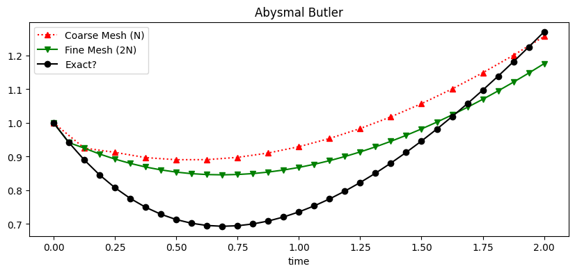
../_images/012f7d0674d224b011c8dcdcfb170ce9aee05ec4ee835fca070361b5760e2fe5.png

Convergent#

The Abysmal-Butler method does satisfy the Lipschitz condition:

(357)#\[\begin{equation}F(t,w:h)-F(t,\hat{w}:h)=\frac{4}{2}f(t,w_i)-\frac{3}{2}f(t-h,w_{i-1}))-(\frac{4}{2}f(t,\hat{w}_{i})-\frac{3}{2}f(t-h,\hat{w}_{i-1})))\end{equation}\]

(358)#\[\begin{equation}F(t,w:h)-F(t,\hat{w}:h)=\frac{4}{2}(f(t,w_i)-f(t,\hat{w}_i))-\frac{3}{2}(f(t-h,w_{i-1}))-f(t-h,\hat{w}_{i-1})))\end{equation}\]

(359)#\[\begin{equation}F(t,w:h)-F(t,\hat{w}:h)\leq\frac{4}{2}L|w_i-\hat{w_i}|+\frac{3}{2}L|w-\hat{w}|\leq \frac{7}{2} L|w_i-\hat{w_i}|\end{equation}\]

This means it is internally convergent,

(360)#\[\begin{equation}|w_i-\hat{w_i}|\rightarrow 0\end{equation}\]

as $h \rightarrow 0$, but as it is not consistent it will never converge to the exact solution

(361)#\[\begin{equation} |y_i-w_i| \not= 0.\end{equation}\]

d = {'time': t[0:5], 'Abysmal Butler': w[0:5],'Abysmal Butler w2 N*2': w2[0:10:2],
     'w-w2':np.abs(w[0:5]-w2[0:10:2])}
df = pd.DataFrame(data=d)
df

	time	Abysmal Butler	Abysmal Butler w2 N*2	w-w2
0	0.000	1.000000	1.000000	0.000000
1	0.125	0.925223	0.925223	0.000000
2	0.250	0.912667	0.892595	0.020072
3	0.375	0.897042	0.869112	0.027930
4	0.500	0.890782	0.853975	0.036807