Example 4th order Runge Kutta

Example 4th order Runge Kutta#

The general form of the population growth differential equation

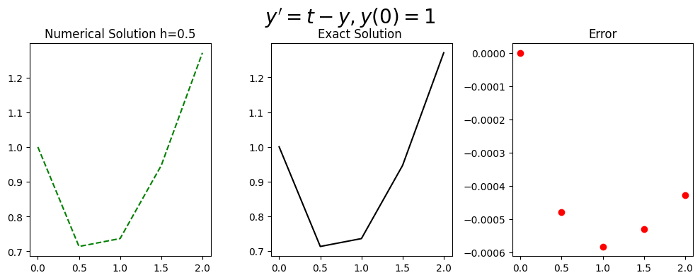
(114)#\[\begin{equation} y^{'}=t-y, \ \ (0 \leq t \leq 2) \end{equation}\]

with the initial condition

(115)#\[\begin{equation}y(0)=1,\end{equation}\]

Has the exact soulation. \begin{equation} y= 2e^{-t}+t-1.\end{equation}

Setting up Libraries#

import numpy as np
import math 

%matplotlib inline
import matplotlib.pyplot as plt # side-stepping mpl backend
import matplotlib.gridspec as gridspec # subplots
import warnings

warnings.filterwarnings("ignore")

Defining the function#

(116)#\[\begin{equation}f(t,y)=t-y\end{equation}\]

def myfun_ty(t,y):
    return t-y

Initial Setup#

Defining the step size \(h\) from the interval range \(a\leq t \leq b\) and number of steps \(N\)

(117)#\[\begin{equation}h=\frac{b-a}{h}.\end{equation}\]

This gives the discrete time steps,

(118)#\[\begin{equation}t_{i}=t_0+ih,\end{equation}\]

where \(t_0=a\).

# Start and end of interval
b=2
a=0
# Step size
N=4
h=(b-a)/(N)
t=np.arange(a,b+h,h)

Setting up the initial conditions of the equation#

(119)#\[\begin{equation}w_0=IC\end{equation}\]

# Initial Condition
IC=1
w=np.zeros(N+1)
y=(IC+1)*np.exp(-t)+t-1#np.zeros(N+1)
w[0]=IC

4th Order Runge Kutta#

(120)#\[\begin{equation}k_1=f(t,y),\end{equation}\]

(121)#\[\begin{equation}k_2=f(t+\frac{h}{2},y+\frac{h}{2}k_2),\end{equation}\]

(122)#\[\begin{equation}k_3=f(t+\frac{h}{2},y+\frac{h}{2}k_2),\end{equation}\]

(123)#\[\begin{equation}k_4=f(t+\frac{h}{2},y+\frac{h}{2}k_3),\end{equation}\]

(124)#\[\begin{equation}w_{i+1}=w_{i}+\frac{h}{6}(k_1+2k_2+2k_3+k_4).\end{equation}\]

for k in range (0,N):
    k1=myfun_ty(t[k],w[k])
    k2=myfun_ty(t[k]+h/2,w[k]+h/2*k1)
    k3=myfun_ty(t[k]+h/2,w[k]+h/2*k2)
    k4=myfun_ty(t[k]+h,w[k]+h*k3)
    w[k+1]=w[k]+h/6*(k1+2*k2+2*k3+k4)

Plotting Results#

fig = plt.figure(figsize=(10,4))
# --- left hand plot
ax = fig.add_subplot(1,3,1)
plt.plot(t,w, '--',color='green')
#ax.legend(loc='best')
plt.title('Numerical Solution h=%s'%(h))

ax = fig.add_subplot(1,3,2)
plt.plot(t,y,color='black')
plt.title('Exact Solution ')

ax = fig.add_subplot(1,3,3)
plt.plot(t,y-w, 'o',color='red')
plt.title('Error')
# --- title, explanatory text and save
fig.suptitle(r"$y'=t-y,   y(0)=%s$"%(IC), fontsize=20)
plt.tight_layout()
plt.subplots_adjust(top=0.85)    

../_images/0b2828aab9175c7207a44f6dbcbe24180d47169d3f0382edb236de9406b0e1be.png

import pandas as pd
d = {'time t_i': t, '4th Order Runge Kutta, w_i': w,'Exact':y,'Error |w-y|':np.round(np.abs(y-w),5)}
df = pd.DataFrame(data=d)
df

	time t_i	4th Order Runge Kutta, w_i	Exact	Error \|w-y\|
0	0.0	1.000000	1.000000	0.00000
1	0.5	0.713542	0.713061	0.00048
2	1.0	0.736342	0.735759	0.00058
3	1.5	0.946791	0.946260	0.00053
4	2.0	1.271100	1.270671	0.00043