Non-Linear Shooting Method

John S Butler john.s.butler@tudublin.ie Course Notes Github

Overview

This notebook illustates the implentation of a the non-linear shooting method to a non-linear boundary value problem.

The non-linear shooting method is a bit like the game Angry Birds to make a first guess and then you refine. The video below walks through the code.

from IPython.display import HTML
HTML('<iframe width="560" height="315" src="https://www.youtube.com/embed/B7MQe09lDC4" frameborder="0" allow="accelerometer; autoplay; clipboard-write; encrypted-media; gyroscope; picture-in-picture" allowfullscreen></iframe>')

/Users/johnbutler/opt/anaconda3/lib/python3.8/site-packages/IPython/core/display.py:724: UserWarning: Consider using IPython.display.IFrame instead
  warnings.warn("Consider using IPython.display.IFrame instead")

Introduction

To numerically approximate the non-linear Boundary Value Problem

(470)\[\begin{equation} y^{''}=f(x,y,y^{'}), \ \ \ a < x < b, \end{equation}\]

with the boundary conditions \begin{equation}y(a)=\alpha,\end{equation} and

(471)\[\begin{equation}y(b) =\beta,\end{equation}\]

using the non-linear shooting method, the Boundary Value Problem is divided into two Initial Value Problems:

1. The first 2nd order non-linear Initial Value Problem is the same as the original Boundary Value Problem with an extra initial condtion \(y_1^{'}(a)=\lambda_0\).

(472)\[\begin{equation} y^{''}_1=f(x,y,y^{'}), \ \ y_1(a)=\alpha, \ \ \color{red}{y^{'}_1(a)=\lambda_0},\\ \end{equation}\]

2. The second 2nd order Initial Value Problem is with respect to \(z=\frac{\partial y}{\partial \lambda}\) with the initial condtions \(z(a)=0\) and \(z^{'}(a)=1\).

(473)\[\begin{equation} z^{''}=\frac{\partial f}{\partial y^{'}}z^{'}(x,\lambda)+\frac{\partial f}{\partial y}z(x,\lambda), \ \ \color{green}{z(a)=0, \ \ z^{'}(a)=1}. \end{equation}\]

combining these results together to get the unique solution

(474)\[\begin{equation} y(x)=y_1(x). \end{equation}\]

Unlike the linear method, the non-linear shooting method is iterative to get the value of \(\lambda\) that results in the same solution as the Boundary Value Problem.

The first choice of \(\lambda_0\) is a guess, then after the first iteration a Newton Raphson method is used to update \(\lambda,\)

(475)\[\begin{equation}\lambda_k=\lambda_{k-1}-\frac{y_1(b,\lambda_{k-1})-\beta}{\frac{dy}{d \lambda}(b,\lambda_{k-1})},\end{equation}\]

which can be re-written as,

(476)\[\begin{equation}\lambda_k=\lambda_{k-1}-\frac{y_1(b,\lambda_{k-1})-\beta}{z(b,\lambda_{k-1})},\end{equation}\]

until \(|\lambda_{k}-\lambda_{k-1}|<tol\).

The introduction of \(\lambda\) is the introduction of a new variable that motivates the second 2nd order Initial Value Problem.

import numpy as np
import math
import matplotlib.pyplot as plt
import warnings
warnings.filterwarnings("ignore")

Example Non-linear Boundary Value Problem

To illustrate the shooting method we shall apply it to the non-linear Boundary Value Problem:

(477)\[\begin{equation} y^{''}=-2yy^{'}, \end{equation}\]

with boundary conditions

(478)\[\begin{equation}y(0) = -2.5, \end{equation}\]

(479)\[\begin{equation}y(1) = 3. \end{equation}\]

The boundary value problem is broken into two second order Initial Value Problems:

1. The first 2nd order Initial Value Problem is the same as the original Boundary Value Problem with an extra initial condtion \(y^{'}(0)=\lambda_0\).

(480)\[\begin{equation} u^{''} =-2uu', \ \ \ \ u(0)=-2.5, \ \ \ \color{green}{u^{'}(0)=\lambda_0}, \end{equation}\]

which can be written a two first order initial value problems

(481)\[\begin{equation} u_1^{'} =u_2, \ \ \ \ u_1(0)=-2.5, \end{equation}\]

(482)\[\begin{equation} u_2^{'} =-2u_1u_2, \ \ \ \ \color{green}{u_2^{'}(0)=\lambda_0}. \end{equation}\]

2. The second 2nd order Initial Value Problem \(z=\frac{\partial y}{\partial \lambda}\) with the initial condtions \(z(a)=0\) and \(z^{'}(a)=1\).with the initial condtions \(z^{'}(0)=0\) and \(z^{'}(0)=1\).

(483)\[\begin{equation} z^{''} =-2y^{'}z-2yz^{'}, \ \ \ \ \color{green}{z(0)=0}, \ \ \ \color{green}{z^{'}(0)=1} \end{equation}\]

which can be written a two first order initial value problems

(484)\[\begin{equation} z_1^{'} =z_2, \ \ \ \ z_1(0)=0, \end{equation}\]

(485)\[\begin{equation} z_2^{'} =-2u_2z_1-2u_1z_2, \ \ \ \ \color{green}{z_2^{'}(0)=1}. \end{equation}\]

The first choice of \(\lambda\) we guess \(\lambda_0=0.2\). Then after the first iteration a Newton Raphson method is used to update \(\lambda\)

(486)\[\begin{equation}\lambda_k=\lambda_{k-1}-\frac{u_1(1,\lambda_{k-1})-3}{z_1(1,\lambda_{k-1})}\end{equation}\]

until \(\lambda_{k}-\lambda_{k-1}<0.001\).

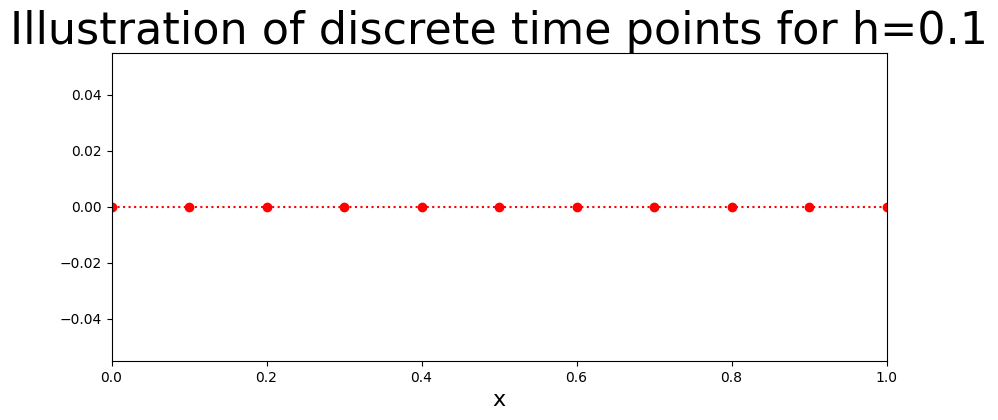
Discrete Axis

The stepsize is defined as

(487)\[\begin{equation}h=\frac{b-a}{N}\end{equation}\]

here it is

(488)\[\begin{equation}h=\frac{1-0}{10}\end{equation}\]

giving

(489)\[\begin{equation}x_i=0+0.1 i\end{equation}\]

for \(i=0,1,...10.\) The plot shows the discrete time intervals.

## BVP
N=10
h=1/N
x=np.linspace(0,1,N+1)
fig = plt.figure(figsize=(10,4))
plt.plot(x,0*x,'o:',color='red')
plt.xlim((0,1))
plt.xlabel('x',fontsize=16)
plt.title('Illustration of discrete time points for h=%s'%(h),fontsize=32)
plt.show()

Initial conditions

The initial conditions for the discrete equations are:

(490)\[\begin{equation} u_1[0]=-2.5\end{equation}\]

(491)\[\begin{equation} u_2[0]=\lambda_0\end{equation}\]

(492)\[\begin{equation} z_1[0]=0\end{equation}\]

(493)\[\begin{equation} z_2[0]=1\end{equation}\]

(494)\[\begin{equation}\beta=3\end{equation}\]

Let \(\lambda_0=0.2\)

U1=np.zeros(N+1)
U2=np.zeros(N+1)
Z1=np.zeros(N+1)
Z2=np.zeros(N+1)

lambda_app=[0.2]
U1[0]=-2.5
U2[0]=lambda_app[0]

Z1[0]=0
Z2[0]=1
beta=3

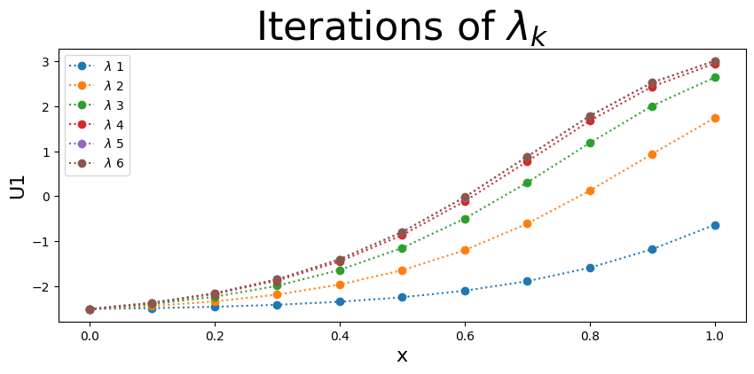
Numerical method

The Euler method is applied to numerically approximate the solution of the system of the two second order non-linear initial value problems they are converted in to two pairs of two first order non-linear initial value problems:

1. Discrete form of Equation 1

(495)\[\begin{equation}u_{1 }[i+1]=u_{1}[i] + h u_{2 }[i]\end{equation}\]

(496)\[\begin{equation}u_{2 }[i+1]=u_{2 }[i] + h (-2u_{1}[i]u_{2 }[i])\end{equation}\]

with the initial conditions \(u_{1}[0]=-2.5\) and \(u_{2}[0]=\lambda_0.\)

2. Discrete form of Equation 2

(497)\[\begin{equation}z_{1}[i+1]=z_{1 }[i] + h z_{2 }[i]\end{equation}\]

(498)\[\begin{equation}z_{2}[i+1]=z_{2 }[i] + h (-2z_{2}[i]y_{1 }[i]-2z_{1 }[i] y_{2 }[i])\end{equation}\]

with the initial conditions \(z_{1}[0]=0\) and \(z_{2}[0]=1\).

At the end of each iteration

(499)\[\begin{equation} u_1[i] \approx y(x_i).\end{equation}\]

The initial choice of \(\lambda_0=0.2\) is up to the user then for each iteration of the system \(\lambda\) is updated using the formula:

(500)\[\begin{equation}\lambda_k=\lambda_{k-1}-\frac{u_1[10]-3}{z_1[10]}.\end{equation}\]

The plot below shows the numerical approximation of the solution to the non-linear Boundary Value Problem for each iteration.

The stopping criteria for the iterative process is

(501)\[\begin{equation}|\lambda_k-\lambda_{k-1}|<tol,\end{equation}\]

with \(tol=0.0001.\)

tol=0.0001
k=0
fig = plt.figure(figsize=(10,4))
while  k<20:
    k=k+1
    for i in range (0,N):
        U1[i+1]=U1[i]+h*(U2[i])
        U2[i+1]=U2[i]+h*(-2*U2[i]*U1[i])
    
        Z1[i+1]=Z1[i]+h*(Z2[i])
        Z2[i+1]=Z2[i]+h*(-2*U2[i]*Z1[i]-2*Z2[i]*U1[i])

    lambda_app.append(lambda_app[k-1]-(U1[N]-beta)/Z1[N])
   
    plt.plot(x,U1,':o',label=r"$\lambda$ %s"%(k))
    plt.xlabel('x',fontsize=16)
    plt.ylabel('U1',fontsize=16)
    U2[0]=lambda_app[k]
    if abs(lambda_app[k]-lambda_app[k-1])<tol:
        break
        
plt.legend(loc='best')
plt.title(r"Iterations of $\lambda_k$",fontsize=32)
plt.show()

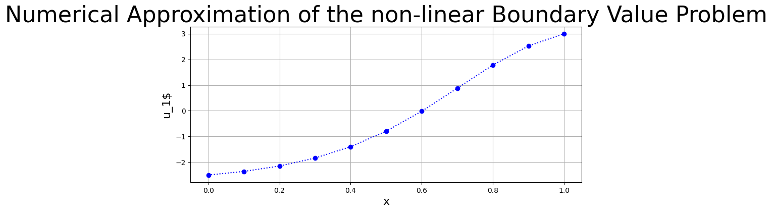
Results

The plot below shows the final iteration of the numerical approximation for the non-linear boundary value problem.

fig = plt.figure(figsize=(10,4))
plt.grid(True)
plt.plot(x,U1,'b:o')
plt.title("Numerical Approximation of the non-linear Boundary Value Problem",fontsize=32)
plt.xlabel('x',fontsize=16)
plt.ylabel("u_1$",fontsize=16)
plt.show()

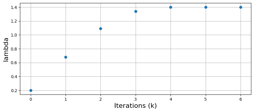
\(\lambda\) Iteration

The plot below shows the iterations of \(\lambda_k\), after \(4\) iterations the value of \(\lambda\) stabilies.

fig = plt.figure(figsize=(10,4))
plt.grid(True)
plt.plot(lambda_app,'o')
#plt.title("Values of $\lambda$ for each interation ",fontsize=32)
plt.xlabel('Iterations (k)',fontsize=16)
plt.ylabel("lambda",fontsize=16)
plt.show()