Universal Approximation Theorem in Action

The code below use a single layer ANN to approximate a sinewave.

Statement of Proof for Sinewave

Let \( C(X,\mathbb{R})\) denote the set of continuous functions from a subset \(X\) of a Euclidean \(\mathbb{R} \)space to a Euclidean space \(\mathbb{R}^.\) Let \(\sigma\) be any continuous sigmoidal function. Then the finite sums of the form:

\[G(\vec{x})=\Sigma_{j=1}^N \alpha_j\sigma(w_j\cdot x+b_j),\]

are dense in \(C([0,1]^n)\). In other words, given any \(f\in C([0,1]^n)\) and \(\epsilon >0\), there is a sum \(G(\vec{x})\) of the above form, for which:

\[|G(x)-sin(x) |<\epsilon,\]

for all \(x\).

import torch
import torch.nn as nn
import torch.optim as optim
import numpy as np
import matplotlib.pyplot as plt

# Generate synthetic data (sine wave)
x = np.linspace(0, 2 * np.pi, 100)  # Input values
y = np.sin(x)  # Target sine wave

# Convert data to PyTorch tensors
x_tensor = torch.FloatTensor(x).unsqueeze(1)  # Reshape to (100, 1)
y_tensor = torch.FloatTensor(y).unsqueeze(1)

    
# Define a simple neural network
class SimpleNN(nn.Module):
    def __init__(self,n_hidden=3):
        super(SimpleNN, self).__init__()
        self.fc1 = nn.Linear(1, n_hidden)  # Input: 1, Hidden: ?
        self.fc2 = nn.Linear(n_hidden, 1)  # Hidden: ?, Output: 1

    def forward(self, x):
        x = torch.sigmoid(self.fc1(x))
        x = self.fc2(x)
        return x

# Instantiate the model, loss function, and optimizer
model = SimpleNN(3)
criterion = nn.MSELoss()
optimizer = optim.Adam(model.parameters(), lr=0.01)
model

SimpleNN(
  (fc1): Linear(in_features=1, out_features=3, bias=True)
  (fc2): Linear(in_features=3, out_features=1, bias=True)
)

Three Node Network

EPOCH=[]
EPOCH_LOSS=[]
# Training the model
num_epochs = 2000
for epoch in range(num_epochs):
    # Forward pass
    outputs = model(x_tensor)
    
    # Compute loss
    loss = criterion(outputs, y_tensor)
    
    # Backpropagation and optimization
    optimizer.zero_grad()
    loss.backward()
    optimizer.step()
    
    if (epoch + 1) % 100 == 0:
        print(f'Epoch [{epoch + 1}/{num_epochs}], Loss: {loss.item():.4f}')
        EPOCH.append(epoch)
        EPOCH_LOSS.append(loss.item())

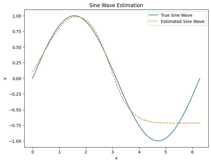
# Plot the estimated sine wave
model.eval()  # Switch to evaluation mode
with torch.no_grad():
    predicted = model(x_tensor).numpy()

plt.figure(figsize=(8, 6))
plt.plot(x, y, label='True Sine Wave')
plt.plot(x, predicted, label='Estimated Sine Wave', linestyle='--')
plt.legend()
plt.xlabel('x')
plt.ylabel('y')
plt.title('Sine Wave Estimation')
plt.show()

Epoch [100/2000], Loss: 0.2096
Epoch [200/2000], Loss: 0.1869
Epoch [300/2000], Loss: 0.1668
Epoch [400/2000], Loss: 0.1017
Epoch [500/2000], Loss: 0.0537
Epoch [600/2000], Loss: 0.0433

Epoch [700/2000], Loss: 0.0412
Epoch [800/2000], Loss: 0.0403
Epoch [900/2000], Loss: 0.0396
Epoch [1000/2000], Loss: 0.0391
Epoch [1100/2000], Loss: 0.0386
Epoch [1200/2000], Loss: 0.0381

Epoch [1300/2000], Loss: 0.0376
Epoch [1400/2000], Loss: 0.0373
Epoch [1500/2000], Loss: 0.0370
Epoch [1600/2000], Loss: 0.0368
Epoch [1700/2000], Loss: 0.0366
Epoch [1800/2000], Loss: 0.0364

Epoch [1900/2000], Loss: 0.0361
Epoch [2000/2000], Loss: 0.0357

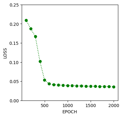
plt.figure(figsize=(4, 4))
plt.plot(EPOCH,EPOCH_LOSS,':og')
plt.ylim((0,0.25))
plt.xlabel('EPOCH')
plt.ylabel('LOSS')
plt.show()

LOSS=[]
for n in range(1,9,1):
    model = SimpleNN(n)
    criterion = nn.MSELoss()
    optimizer = optim.Adam(model.parameters(), lr=0.01)
    # Training the model
    num_epochs = 2000

    for epoch in range(num_epochs):
        # Forward pass
        outputs = model(x_tensor)

        # Compute loss
        loss = criterion(outputs, y_tensor)

        # Backpropagation and optimization
        optimizer.zero_grad()
        loss.backward()
        optimizer.step()

        if (epoch + 1) % 1000 == 0:
            print(f'Node [{n}], Epoch [{epoch + 1}/{num_epochs}], Loss: {loss.item():.4f}')
    LOSS.append(loss.item())
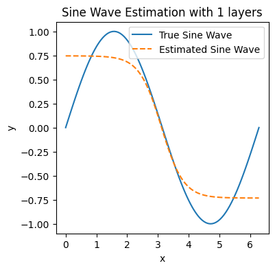
        # Plot the estimated sine wave
    model.eval()  # Switch to evaluation mode
    with torch.no_grad():
        predicted = model(x_tensor).numpy()

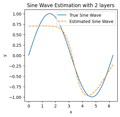
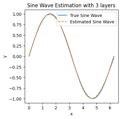
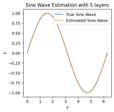
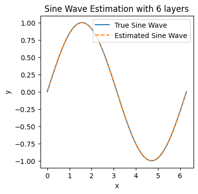
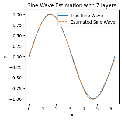
    plt.figure(figsize=(4, 4))
    plt.plot(x, y, label='True Sine Wave')
    plt.plot(x, predicted, label='Estimated Sine Wave', linestyle='--')
    plt.legend()
    plt.xlabel('x')
    plt.ylabel('y')
    plt.title('Sine Wave Estimation with '+str(n)+' layers')
    plt.show()

Node [1], Epoch [1000/2000], Loss: 0.0904

Node [1], Epoch [2000/2000], Loss: 0.0721

Node [2], Epoch [1000/2000], Loss: 0.0790

Node [2], Epoch [2000/2000], Loss: 0.0388

Node [3], Epoch [1000/2000], Loss: 0.0075

Node [3], Epoch [2000/2000], Loss: 0.0003

Node [4], Epoch [1000/2000], Loss: 0.0113

Node [4], Epoch [2000/2000], Loss: 0.0002

Node [5], Epoch [1000/2000], Loss: 0.0008

Node [5], Epoch [2000/2000], Loss: 0.0001

Node [6], Epoch [1000/2000], Loss: 0.0007

Node [6], Epoch [2000/2000], Loss: 0.0000

Node [7], Epoch [1000/2000], Loss: 0.0350

Node [7], Epoch [2000/2000], Loss: 0.0005

Node [8], Epoch [1000/2000], Loss: 0.0003

Node [8], Epoch [2000/2000], Loss: 0.0000

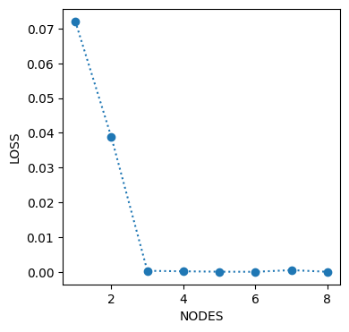
plt.figure(figsize=(4, 4))
plt.plot(np.arange(1,9),LOSS,':o')

plt.xlabel('NODES')
plt.ylabel('LOSS')
plt.show()

Ten Node Network

EPOCH10=[]
EPOCH10_LOSS=[]
model = SimpleNN(10)
criterion = nn.MSELoss()
optimizer = optim.Adam(model.parameters(), lr=0.01)
# Training the model
num_epochs = 2000
for epoch in range(num_epochs):
    # Forward pass
    outputs = model(x_tensor)
    
    # Compute loss
    loss = criterion(outputs, y_tensor)
    
    # Backpropagation and optimization
    optimizer.zero_grad()
    loss.backward()
    optimizer.step()
    
    if (epoch + 1) % 100 == 0:
        print(f'Epoch [{epoch + 1}/{num_epochs}], Loss: {loss.item():.4f}')
        EPOCH10.append(epoch)
        EPOCH10_LOSS.append(loss.item())

# Plot the estimated sine wave
model.eval()  # Switch to evaluation mode
with torch.no_grad():
    predicted = model(x_tensor).numpy()

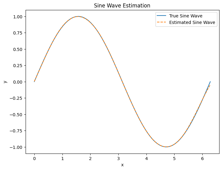
plt.figure(figsize=(8, 6))
plt.plot(x, y, label='True Sine Wave')
plt.plot(x, predicted, label='Estimated Sine Wave', linestyle='--')
plt.legend()
plt.xlabel('x')
plt.ylabel('y')
plt.title('Sine Wave Estimation')
plt.show()

Epoch [100/2000], Loss: 0.1995
Epoch [200/2000], Loss: 0.1840
Epoch [300/2000], Loss: 0.1598
Epoch [400/2000], Loss: 0.0919
Epoch [500/2000], Loss: 0.0423
Epoch [600/2000], Loss: 0.0334

Epoch [700/2000], Loss: 0.0267
Epoch [800/2000], Loss: 0.0191
Epoch [900/2000], Loss: 0.0121
Epoch [1000/2000], Loss: 0.0070
Epoch [1100/2000], Loss: 0.0040
Epoch [1200/2000], Loss: 0.0024

Epoch [1300/2000], Loss: 0.0015
Epoch [1400/2000], Loss: 0.0009
Epoch [1500/2000], Loss: 0.0005
Epoch [1600/2000], Loss: 0.0003
Epoch [1700/2000], Loss: 0.0002
Epoch [1800/2000], Loss: 0.0001

Epoch [1900/2000], Loss: 0.0001
Epoch [2000/2000], Loss: 0.0000

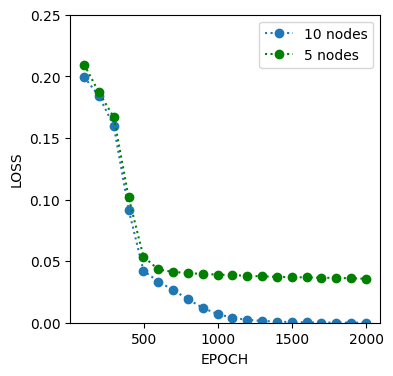
plt.figure(figsize=(4, 4))
plt.plot(EPOCH10,EPOCH10_LOSS,':o',label='10 nodes')
plt.plot(EPOCH,EPOCH_LOSS,':og',label='5 nodes')
plt.ylim((0,0.25))
plt.xlabel('EPOCH')
plt.ylabel('LOSS')
plt.legend()
plt.show()