Question 6 Integrate and Fire

from IPython.display import YouTubeVideo

YouTubeVideo('KDQpwb8MSOc', width=800, height=300)

YouTubeVideo('VSJvHiw6oo8', width=800, height=300)

Approximate the solution of the integrate and fire differential equation:

(566)\[\begin{equation} \tau_m\frac{dV}{dt} = -(V-E_L) + R_mI(t), \ \ -50\leq t \leq 400, \end{equation}\]

where \(E_L = -75\), \(\tau_m = 10\), \(R_m = 10\) and \(I(t)=0.01t\) and the initial condition \(V(-50) = -75\) using a stepsize of \(h=0.5\). Using the:

1. Euler Method;

2. 2nd Order Taylor Method;

3. Heun’s Method (2nd Order Runge Kutta);

4. 2-step Adams Bashforth Method.

## Library
import numpy as np

%matplotlib inline
import matplotlib.pyplot as plt # side-stepping mpl backend
import matplotlib.gridspec as gridspec # subplots
import warnings

warnings.filterwarnings("ignore")

Discrete Interval

The continuous time \(a\leq t \leq b \) is discretised with stepsize \(h=0.5\) gives

(567)\[\begin{equation} N=\frac{b-a}{h}. \end{equation}\]

Here the N is \(-50\leq t \leq 400\)

(568)\[\begin{equation} N=\frac{400--50}{0.5}=900, \end{equation}\]

this gives the 901 discrete points:

(569)\[\begin{equation} t_0=-400, \ t_1=-399.5, \ ... t_{900}=400. \end{equation}\]

This is generalised to

(570)\[\begin{equation} t_i=-50+i0.1, \ \ \ i=0,1,...,900. \end{equation}\]

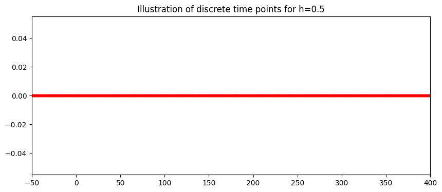
The plot below shows the discrete time steps.

### Setting up time
a=-50 # Start time point
b=400 # end time point
h=0.5 # step size

N=int((b-a)/(h)) # Number of gaps 

t=np.arange(a,b+h/2,h) # -50, 400

fig = plt.figure(figsize=(10,4))
plt.plot(t,0*t,'.',color='red')
plt.xlim((a,b))
plt.title('Illustration of discrete time points for h=%s'%(h))
plt.plot();

Euler Method

The general form of the Euler method is

(571)\[\begin{equation} w_{i+1}=w_{i}+hf(t_i,w_i). \end{equation}\]

The Integrate and fire differential equation is transformed using the Euler method into a difference equation of the form

(572)\[\begin{equation} w_{i+1}=w_{i}+h\big[\frac{-(w_i-E_L) + R_mI(t_i)}{\tau_m}\big] \end{equation}\]

for \(i=0,1,...,899\) and where \(E_L = -75\), \(\tau_m = 10\), \(R_m = 10\) and \(I(t_i)=0.01t_i\) and the initial condition \(V(t_0=-50) = -75\) using a stepsize of \(h=0.5\). Putting in the values the difference equation is

(573)\[\begin{equation} w[i+1]=w[i]+0.5\big[-(w[i]--75) + 10*0.01*t[i]\big]/10 \end{equation}\]

(574)\[\begin{equation} \color{red}{w[i+1]}=\color{green}{w[i]}+0.5\big(-(\color{red}{w[i]}+75) + 0.1*t[i]\big)/10 .\end{equation}\]

In the solution, I will use Euler for Euler approximation, which gives:

(575)\[\begin{equation} \color{red}{Euler[i+1]}=\color{green}{Euler[i]}+0.5\big(-(\color{red}{Euler[i]}+75) + 0.1*t[i]\big)/10. \end{equation}\]

Euler=np.zeros(N+1) # list of 901 0s
Euler[0]=-75 ## INITIAL CONDITION
for i in range (0,N): # 0,1,...899
    Euler[i+1]=Euler[i]+h*(-(Euler[i]+75)+0.1*t[i])/10

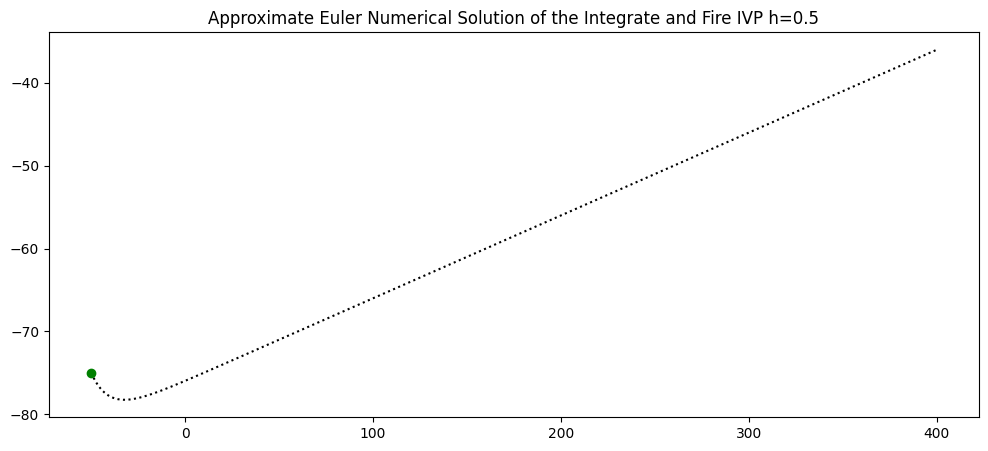
fig = plt.figure(figsize=(12,5))
plt.plot(t,Euler,':',color='k')
plt.plot(t[0],Euler[0],'o',color='green')
plt.title('Approximate Euler Numerical Solution of the Integrate and Fire IVP h=%s'%(h))
plt.show()

For simpilicty of numerical implimentation of the integrate and fire differential equation:

(576)\[\begin{equation} \tau_m\frac{dV}{dt} = -(V-E_L) + R_mI(t), \end{equation}\]

we re-arranged as:

(577)\[\begin{equation} \frac{dV}{dt} =f_{IF}(t,V), \end{equation}\]

where

(578)\[\begin{equation} f_{IF}(t,V) = \frac{-(V-E_L) + R_mI(t)}{\tau_m}.\end{equation}\]

# definint a function for f_IF that takes in t and V
def f_IF(t,V):
    R_m=10
    tau_m=10
    E_L=-75
    I=0.01*t
    f=(-(V-E_L)+R_m*I)/tau_m
    return f

2nd Order Taylor

The general 2nd Order Taylor method for to the first order differential equation

(579)\[\begin{equation} y^{'} = f(t,y), \end{equation}\]

numerical approximates \(y\) the at time point \(t_i\) as \(w_i\) with the formula:

(580)\[\begin{equation} w_{i+1}=w_i+h\big[f(t_i,w_i)+\frac{h}{2}f'(t_i,w_i)\big],\end{equation}\]

where \(h\) is the stepsize. for \(i=0,...,N-1\).

For the Integrate and fire:

(581)\[\begin{equation} f_{IF}(t,V) = \frac{-(V-E_L) + R_mI(t)}{\tau_m}.\end{equation}\]

The 2nd Order Taylor will be of the form:

(582)\[\begin{equation} w_{i+1}=w_i+h\big[f_{IF}(t_i,w_i)+\frac{h}{2}f'_{IF}(t_i,w_i)\big]. \end{equation}\]

We need to get \(f_{IF}'\):

(583)\[\begin{equation} f_{IF}'(t,V) = \frac{-(V'-0) + R_mI'(t)}{\tau_m}.\end{equation}\]

by definition of the IVP we have:

(584)\[\begin{equation} V'(t)=f_{IF}(t,V) = \frac{-(V-E_L) + R_mI(t)}{\tau_m}\end{equation}\]

and \(I(t)=0.01t\)

(585)\[\begin{equation} I'(t)=0.01.\end{equation}\]

In the solution, I will use Taylor for Taylor approximation, which gives:

(586)\[\begin{equation} \color{red}{Taylor[i+1]}=\color{green}{Taylor[i]}+0.5f_{IF}(t[i],\color{green}{Taylor[i]})+\frac{0.5^2}{2}f'_{IF}(t[i],\color{green}{Taylor[i]}) \end{equation}\]

which gives:

(587)\[\begin{equation} \color{red}{Taylor[i+1]}=\color{green}{Taylor[i]}+0.5f_{IF}(t[i],\color{green}{Taylor[i]})+\frac{0.5^2}{2}(-f_{IF}(t[i],\color{green}{Taylor[i]})/\tau_m+0.1/\tau_m) \end{equation}\]

Taylor=np.zeros(N+1)
Taylor[0]=-75 ## INITIAL CONDITION
for i in range (0,N):
## ADD EQUATION DYNAMICS TO EQUATION
    Taylor[i+1]=Taylor[i]+h*f_IF(t[i],Taylor[i])+h*h/2*(-f_IF(t[i],Taylor[i])/10+0.1/10)

Heun’s Method (2nd Order Runge Kutta)

The general Heun’s method for to the first order differential equation

(588)\[\begin{equation} y^{'} = f(t,y) \end{equation}\]

numerical approximates \(y\) the at time point \(t_i\) as \(w_i\) with the formula:

(589)\[\begin{equation} w_{i+1}=w_i+\frac{h}{2}\big[k_1+k_2],\end{equation}\]

for \(i=0,...,N-1\), where

(590)\[\begin{equation}k_1=f(t_i,w_i),\end{equation}\]

and

(591)\[\begin{equation}k_2=f(t_i+h,w_i+hk_1),\end{equation}\]

and \(h\) is the stepsize.

In the solution, I will use Huen for Heun approximation, which gives:

(592)\[\begin{equation} Heun[i+1]=Huen[i]+\frac{h}{2}\big[k_1+k_2],\end{equation}\]

for \(i=0,...,N-1\), where

(593)\[\begin{equation}k_1=f_{IK}(t[i],Huen[i]),\end{equation}\]

and

(594)\[\begin{equation}k_2=f_{IK}(t[i]+h,Heun[i]+hk_1),\end{equation}\]

and \(h\) is the stepsize.

Heun=np.zeros(N+1)
Heun[0]=-75 ## INITIAL CONDITION
for i in range (0,N):
## ADD EQUATION DYNAMICS TO EQUATION
    k1=f_IF(t[i],Heun[i])
    k2=f_IF(t[i]+h,Heun[i]+h*k1)
    Heun[i+1]=Heun[i]+h/2*(k1+k2)

2-step Adams-Bashforth

The general 2-step Adams-Bashforth method for the first order differential equation

(595)\[\begin{equation} y^{'} = f(t,y), \end{equation}\]

numerical approximates \(y\) the at time point \(t_i\) as \(w_i\) with the formula:

(596)\[\begin{equation} w_{i+1}=w_i+\frac{h}{2}\big[3f(t_i,w_i)-f(t_{i-1},w_{i-1})\big],\end{equation}\]

for \(i=1,...,N-1\), where

and \(h\) is the stepsize.

For the Integrate and Fire Equation we have

(597)\[\begin{equation} w_{i+1}=w_i+\frac{h}{2}\big[3f_{IF}(t_i,w_i)-f_{IF}(t_{i-1},w_{i-1})\big],\end{equation}\]

I will use AB to denote the approximate from the 2-step Adams-Bashforth:

(598)\[\begin{equation} AB[i+1]=AB[i]+\frac{h}{2}\big[3f_{IF}(t[i],AB[i])-f_{IF}(t[i-1],AB[i-1])\big],\end{equation}\]

for \(i=1,...,899\). We need to approximate \(AB[1]\) for the 2-step method. Here I will use the Heun solution at the second step i=1.

AB=np.zeros(N+1)
AB[0]=-75 ## INITIAL CONDITION
AB[1]=Heun[1] ## INITIAL HUEN CONDITION
for i in range (1,N):
    AB[i+1]=AB[i]+h/2*(3*f_IF(t[i],AB[i])-f_IF(t[i-1],AB[i-1]))

fig = plt.figure(figsize=(12,5))

plt.plot(t,Euler,':',color='k',label='Euler')
plt.plot(t,Taylor,':',color='r',label='Taylor')
plt.plot(t,Heun,':',color='b',label='Heun')
plt.plot(t,AB,':',color='g',label='Adams-Bashforth')

plt.plot(t[0],Euler[0],'o',color='black',label='Initial Condition')

plt.legend(loc='best')
plt.xlabel('time (ms)')
plt.ylabel('Voltage')
plt.title('Numerical Solutions h=%s'%(h))
plt.show()

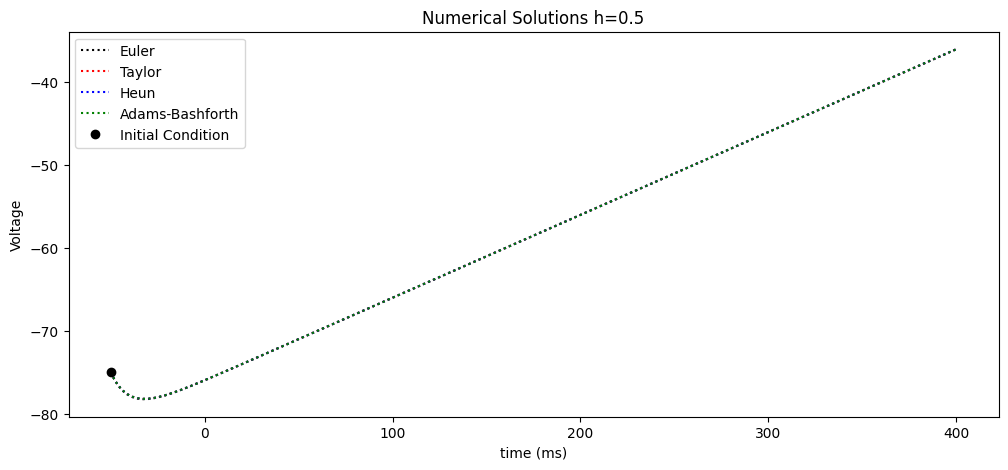
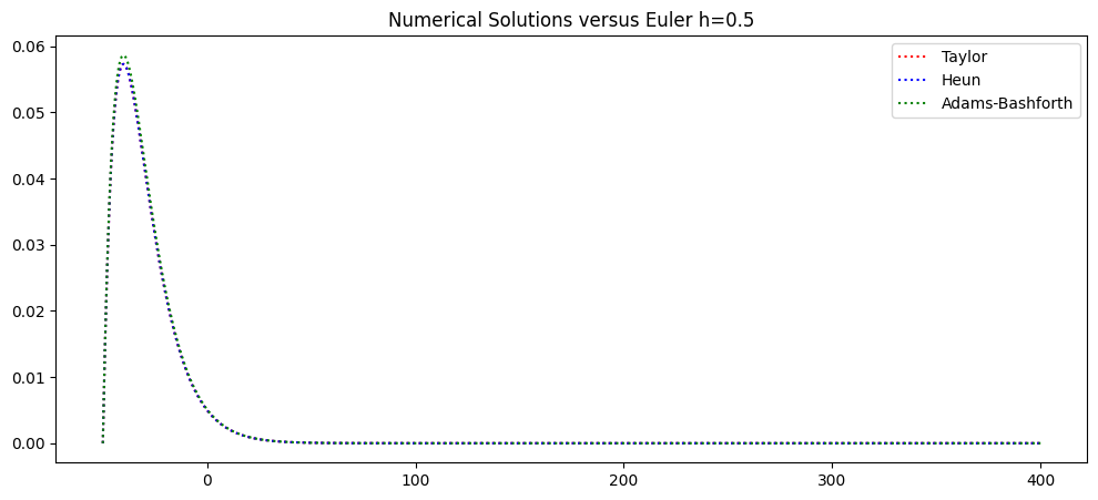
fig = plt.figure(figsize=(12,5))

plt.plot(t,Taylor-Euler,':',color='r',label='Taylor')
plt.plot(t,Heun-Euler,':',color='b',label='Heun')
plt.plot(t,AB-Euler,':',color='g',label='Adams-Bashforth')


plt.legend(loc='best')
plt.title('Numerical Solutions versus Euler h=%s'%(h))
plt.show()