Gradient Descent#
Gradient descent is an iterative optimization algorithm used to minimize a cost or loss function by adjusting the parameters of a model or system. The basic idea behind gradient descent is to move in the direction of steepest descent (the negative gradient) of the cost function to reach a local or global minimum.
Given a cost or loss function, denoted as \(J(\theta)\), where \(\theta\) represents a set of parameters that you want to optimize. The goal is to find the values of \(\theta\) that minimize \(J(\theta)\).
Initialization: Start with an initial guess for the parameters, \(\theta_0\). Typically, \(\theta_0\) is initialized randomly or with some predetermined values.
Update Rule: In each iteration, you update the parameters \(\theta\) as follows:
\[ \theta_{i+1} = \theta_i - \alpha \nabla J(\theta_i) \]where:
\(\theta_i\) is the current set of parameters.
\(\alpha\) (alpha) is the learning rate, a hyperparameter that determines the step size in the direction of the gradient.
\(\nabla J(\theta_i)\) is the gradient of the cost function with respect to the parameters \(\theta\).
Stopping Criterion: You continue to update the parameters using the update rule until a stopping criterion is met. Common stopping criteria include:
A maximum number of iterations.
Achieving a satisfactory level of convergence, which can be defined as a small change in the cost function or a small change in the parameters.
Optimal Parameters: The final values of \(\theta\) obtained after the algorithm converges are the optimal parameters that minimize the cost function:
The key to gradient descent is the calculation of the gradient \(\nabla J(\theta)\), which represents the direction of the steepest ascent of the cost function at the current parameter values. The negative gradient \(-\nabla J(\theta)\) points in the direction of the steepest descent, which is the direction in which you adjust the parameters to reduce the cost function.
It’s important to choose an appropriate learning rate (\(\alpha\)) for gradient descent. If \(\alpha\) is too small, the algorithm may converge very slowly, while if it’s too large, it may fail to converge or even diverge. Finding the right learning rate is often an empirical process and can be a challenge in practice.
Gradient descent is a fundamental optimization algorithm used in various machine learning and optimization tasks, including training machine learning models (e.g., linear regression, neural networks), solving linear systems, and more.
import numpy as np
import matplotlib.pyplot as plt
Example Code#
Given simple quadratic cost function
for which we want to find the minimum.
# Define the quadratic function J(\theta) = \theta^2+2\theta+100
def quadratic_cost_function(theta):
    return theta**2+2*theta+100
The gradient of the function,
which is used in the gradient descent update.
# Define the derivative of the quadratic function f'(x) = 2x
def gradient(theta):
    return 2 * theta+2
The learning rate \(\alpha\) and the number of max iterations for the gradient descent.
# Gradient Descent parameters
learning_rate = 0.1  # Step size or learning rate
Choose an initial guess for \( \theta_0 \).
# Initial guess
theta_0 = 10.0
The gradient descent function iteratively updates \( \theta \) using the gradient and learning rate and appends the updated values to the history lists,
def gradient_descent(theta,learning_rate=0.1, tol=1e-6, max_iter=100):
    theta_history = [theta]
    cost_history = [quadratic_cost_function(theta)]
    for i in range(max_iter):
        # Update x using the gradient and learning rate
        theta_new = theta - learning_rate * gradient(theta)

        # Append the updated values to the history lists
        theta_history.append(theta_new)
        cost_history.append(quadratic_cost_function(theta_new))
        if abs(theta-theta_new) < tol:
            return theta,theta_history, cost_history,i
        theta=theta_new

    return theta,theta_history, cost_history,i
Choose the stopping criteria tol and max iteratinos such that the algorithms stops when the parameter converges to within a tolerance
or the number of iterations reaches the max iterations.
tol=0.001
max_iterations = 100     # Number of iterations
Run the function and print the optimal value found by gradient descent of \( \theta \), the minimum value of the cost function \( J(\theta) \) and the number of iterations \(I\).
theta, theta_history, cost_history,I=gradient_descent(theta_0,learning_rate=learning_rate,tol=tol,max_iter=max_iterations)
# Print the final result
print(f'Optimal theta: {theta}')
print(f"Minimum Cost value: {quadratic_cost_function(theta)}")
print(f"Number of Interations I: {I}")
Optimal theta: -0.9955378698871966
Minimum Cost value: 99.00001991060515
Number of Interations I: 35
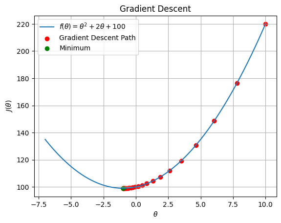
Plotting the function $\( J(\theta) \)$ and the optimization path taken by gradient descent.
# Perform gradient descent
# Plot the function and optimization path

theta_values = np.linspace(-7, 10, 100)
cost_values = quadratic_cost_function(theta_values)


plt.plot(theta_values, cost_values, label=r'$f(\theta) = \theta^2+2\theta+100$')
plt.scatter(theta_history, cost_history, c='red', label='Gradient Descent Path')
plt.scatter(theta, quadratic_cost_function(theta), c='g', label='Minimum')
plt.xlabel(r'$\theta$')
plt.ylabel(r'$J(\theta)$')
plt.legend()
plt.grid(True)
plt.title('Gradient Descent')
plt.show()
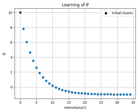
Plotting \( \theta \) as a function of itertations (i).
plt.scatter(0,theta_history[0],  c='k', label='Initial Guess')
plt.plot(np.arange(1,I),theta_history[1:I],'o')
plt.xlabel(r'$Interations (i)$')
plt.ylabel(r'$\theta_i$')
plt.legend()
plt.grid(True)
plt.title(r'Learning of $\theta$')
plt.show()
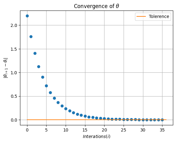
Showing the converge of \(\theta\) by plotting \(|\theta_{i+1}-\theta_{i}|\) as a function of itertations (i).
plt.plot(np.abs(np.diff(theta_history)),'o')
plt.plot([0,I+1],[tol,tol],label='Tolerence')
plt.xlabel(r'$Interations (i)$')
plt.ylabel(r'$|\theta_{i+1}-\theta_{i}|$')
plt.legend()
plt.grid(True)
plt.title(r'Convergence of $\theta$')
plt.show()
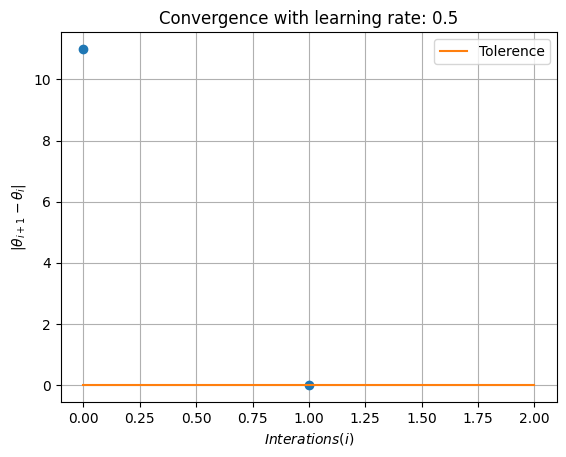
Playing with Learning Rate#
alpha=0.5
theta, theta_history, cost_history,I=gradient_descent(theta_0,learning_rate=alpha,tol=tol,max_iter=max_iterations)
# Print the final result
print(f'Optimal theta: {theta}')
print(f"Minimum Cost value: {quadratic_cost_function(theta)}")
print(f"Number of Interations I: {I}")

plt.plot(np.abs(np.diff(theta_history)),'o')
plt.plot([0,I+1],[tol,tol],label='Tolerence')
plt.xlabel(r'$Interations (i)$')
plt.ylabel(r'$|\theta_{i+1}-\theta_{i}|$')
plt.legend()
plt.grid(True)
plt.title(f'Convergence with learning rate: {alpha}')
plt.show()
Optimal theta: -1.0
Minimum Cost value: 99.0
Number of Interations I: 1
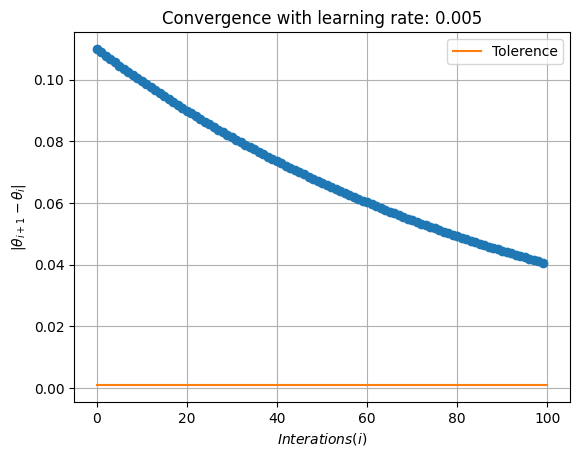
alpha=0.005
theta, theta_history, cost_history,I=gradient_descent(theta_0,learning_rate=alpha,tol=tol,max_iter=max_iterations)
# Print the final result
print(f'Optimal theta: {theta}')
print(f"Minimum Cost value: {quadratic_cost_function(theta)}")
print(f"Number of Interations I: {I}")

plt.plot(np.abs(np.diff(theta_history)),'o')
plt.plot([0,I+1],[tol,tol],label='Tolerence')
plt.xlabel(r'$Interations (i)$')
plt.ylabel(r'$|\theta_{i+1}-\theta_{i}|$')
plt.legend()
plt.grid(True)
plt.title(f'Convergence with learning rate: {alpha}')
plt.show()
Optimal theta: 3.0263557540055266
Minimum Cost value: 115.21154065781342
Number of Interations I: 99