Adams Bashforth

Adams Bashforth#

John S Butler#

john.s.butler@tudublin.ie
Course Notes Github

The Adams Bashforth method is an explicit multistep method. This notebook illustrates the 2 step Adams Bashforth method for a linear initial value problem, given by

(192)#

y^{^{'}} = t - y, (0 \leq t \leq 2)

with the initial condition

(193)#

y (0) = 1.

The video below walks through the notebook.

from IPython.display import HTML
HTML('<iframe width="560" height="315" src="https://www.youtube.com/embed/etob5sngUUc" frameborder="0" allow="accelerometer; autoplay; clipboard-write; encrypted-media; gyroscope; picture-in-picture" allowfullscreen></iframe>')

/Users/johnbutler/opt/anaconda3/lib/python3.8/site-packages/IPython/core/display.py:724: UserWarning: Consider using IPython.display.IFrame instead
  warnings.warn("Consider using IPython.display.IFrame instead")

Python Libraries#

import numpy as np
import math 
import pandas as pd
%matplotlib inline
import matplotlib.pyplot as plt # side-stepping mpl backend
import matplotlib.gridspec as gridspec # subplots
import warnings

warnings.filterwarnings("ignore")

Defining the function#

(194)#

f (t, y) = t - y .

def myfun_ty(t,y):
    return t-y

Discrete Interval#

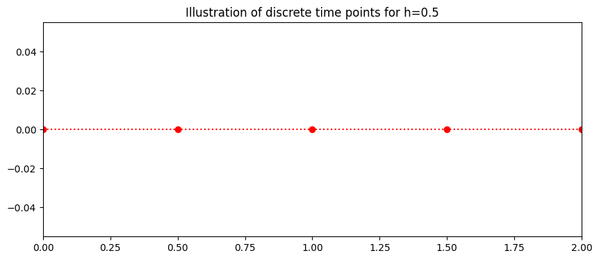
Defining the step size $h$ from the interval range $a \leq t \leq b$ and number of steps $N$

(195)#

h = \frac{b - a}{N} .

This gives the discrete time steps,

(196)#

t_{i} = t_{0} + i h,

where $t 0 = a .$

Here the interval is $0 \leq t \leq 2$ and number of step 4

(197)#

h = \frac{2 - 0}{4} = 0.5 .

This gives the discrete time steps,

(198)#

t_{i} = 0 + i 0.5,

for $i = 0, 1, \dots, 4.$

# Start and end of interval
b=2
a=0
# Step size
N=4
h=(b-a)/(N)
t=np.arange(a,b+h,h)
fig = plt.figure(figsize=(10,4))
plt.plot(t,0*t,'o:',color='red')
plt.xlim((0,2))
plt.title('Illustration of discrete time points for h=%s'%(h))

Text(0.5, 1.0, 'Illustration of discrete time points for h=0.5')

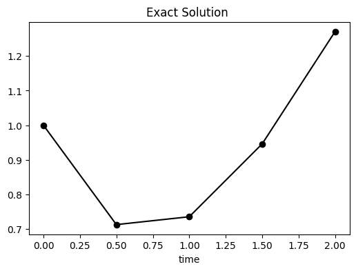
../_images/c8398a8e754352c5ba975132569e814b786f734c1a6a07741fce9c26e38b0946.png

Exact Solution#

THe initial value problem has the exact solution

(199)#

y (t) = 2 e^{- t} + t - 1.

The figure below plots the exact solution.

IC=1 # Intial condtion
y=(IC+1)*np.exp(-t)+t-1
fig = plt.figure(figsize=(6,4))
plt.plot(t,y,'o-',color='black')
plt.title('Exact Solution ')
plt.xlabel('time')

Text(0.5, 0, 'time')

../_images/287b099acfa344ba6bddcd56b3ed6036cfd68f5cecd7382b9b599521edd7a0d0.png

2-step Adams Bashforth#

The general 2-step Adams Bashforth difference equation is

(200)#

w_{i + 1} = w_{i} + \frac{h}{2} (3 f (t_{i}, w_{i}) - f (t_{i - 1}, w_{i - 1})) .

For the specific intial value problem the 2-step Adams Bashforth difference equation is

(201)#

w_{i + 1} = w_{i} + \frac{h}{2} (3 (t_{i} - w_{i}) - (t_{i - 1} - w_{i - 1})) .

for $i = 0$ the difference equation is:

(202)#

w_{1} = w_{0} + \frac{h}{2} (3 (t_{0} - w_{0}) - (t_{- 1} - w_{- 1})),

this is not solvable as $w_{- 1}$ is unknown. for $i = 1$ the difference equation is:

(203)#

w_{2} = w_{1} + \frac{h}{2} (3 (t_{1} - w_{1}) - (t_{0} - w_{0})),

this is not solvable as $w_{1}$ is unknown, but it can be approximated using a one step method. Here, as the exact solution is known,

(204)#

w_{1} = 2 e^{- t_{1}} + t_{1} - 1.

### Initial conditions
w=np.zeros(len(t))
w[0]=IC
w[1]=y[1] # NEED FOR THE METHOD

Loop#

for k in range (1,N):
    w[k+1]=w[k]+h/2.0*(3*myfun_ty(t[k],w[k])-myfun_ty(t[k-1],w[k-1]))   

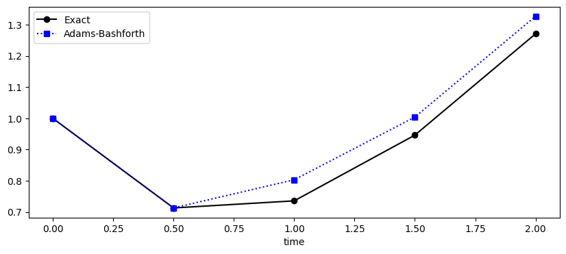
Plotting solution#

def plotting(t,w,y):
    fig = plt.figure(figsize=(10,4))
    plt.plot(t,y, 'o-',color='black',label='Exact')
    plt.plot(t,w,'s:',color='blue',label='Adams-Bashforth')
    plt.xlabel('time')
    plt.legend()
    plt.show 

The plot below shows the exact solution (black) and the 2 step Adams-Bashforth approximation (red) of the intial value problem

plotting(t,w,y)

../_images/a6d7a94fcca546dd1e35f46b0f1cd4c62892277ee282673045e60a663847ca56.png

Local Error#

The Error for the 2 step Adams Bashforth is:

(205)#

y_{n + 1} = y_{n} + \frac{h}{2} [3 f (t_{n}, w_{n}) - f (t_{n - 1}, w_{n - 1})] + \frac{5 h^{3}}{12} y^{‴} (η),

where $η \in [t_{n - 1}, t_{n + 1}]$ .

Rearranging the equations gives

(206)#

\frac{y_{n + 1} - y_{n}}{h} = \frac{1}{2} [3 f (t_{n}, w_{n}) - f (t_{n - 1}, w_{n - 1})] + \frac{5 h^{2}}{12} y^{‴} (η) .

For our specific initial value problem the error is of the form:

(207)#

\frac{5 h^{2}}{12} y^{‴} (η) = \frac{5 h^{2}}{12} 2 e^{- η} \leq \frac{5 (0.5)^{2}}{12} 2 \leq 0.208

d = {'time t_i': t, 'Adams Bashforth, w_i': w,'Exact':y,'Error |w-y|':np.round(np.abs(y-w),5),'LTE':round(2*0.5**2/12*5,5)}
df = pd.DataFrame(data=d)
df

	time t_i	Adams Bashforth, w_i	Exact	Error \|w-y\|	LTE
0	0.0	1.000000	1.000000	0.00000	0.20833
1	0.5	0.713061	0.713061	0.00000	0.20833
2	1.0	0.803265	0.735759	0.06751	0.20833
3	1.5	1.004082	0.946260	0.05782	0.20833
4	2.0	1.326837	1.270671	0.05617	0.20833