Application of 2nd order Runge Kutta to Populations Equations

Application of 2nd order Runge Kutta to Populations Equations#

This notebook implements the 2nd Order Runge Kutta method for three different population intial value problems.

2nd Order Runge Kutta#

The general 2nd Order Runge Kutta method for to the first order differential equation

(134)#\[\begin{equation} y^{'} = f(t,y) \end{equation}\]

numerical approximates \(y\) the at time point \(t_i\) as \(w_i\) with the formula:

(135)#\[\begin{equation} w_{i+1}=w_i+\frac{h}{2}\big[k_1+k_2],\end{equation}\]

for \(i=0,...,N-1\), where

(136)#\[\begin{equation}k_1=f(t_i,w_i),\end{equation}\]

and

(137)#\[\begin{equation}k_2=f(t_i+h,w_i+hk_1),\end{equation}\]

and \(h\) is the stepsize.

To illustrate the method we will apply it to three intial value problems:

1. Linear#

Consider the linear population Differential Equation

(138)#\[\begin{equation} y^{'}=0.1y, \ \ (2000 \leq t \leq 2020), \end{equation}\]

with the initial condition,

(139)#\[\begin{equation}y(2000)=6.\end{equation}\]

2. Non-Linear Population Equation#

Consider the non-linear population Differential Equation

(140)#\[\begin{equation} y^{'}=0.2y-0.01y^2, \ \ (2000 \leq t \leq 2020), \end{equation}\]

with the initial condition,

(141)#\[\begin{equation}y(2000)=6.\end{equation}\]

3. Non-Linear Population Equation with an oscillation#

Consider the non-linear population Differential Equation with an oscillation

(142)#\[\begin{equation} y^{'}=0.2y-0.01y^2+\sin(2\pi t), \ \ (2000 \leq t \leq 2020), \end{equation}\]

with the initial condition,

(143)#\[\begin{equation}y(2000)=6.\end{equation}\]

Setting up Libraries#

## Library
import numpy as np
import math 
import pandas as pd
%matplotlib inline
import matplotlib.pyplot as plt # side-stepping mpl backend
import matplotlib.gridspec as gridspec # subplots
import warnings

warnings.filterwarnings("ignore")

Discrete Interval#

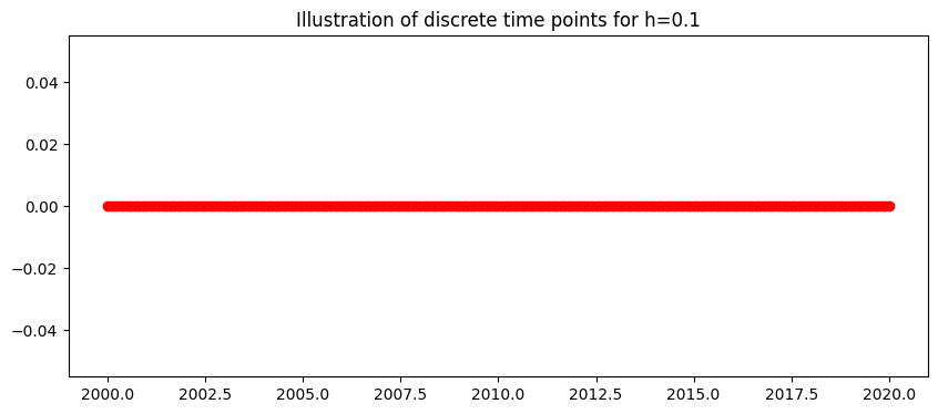
The continuous time \(a\leq t \leq b \) is discretised into \(N\) points seperated by a constant stepsize

(144)#\[\begin{equation} h=\frac{b-a}{N}.\end{equation}\]

Here, the interval is \(2000\leq t \leq 2020,\)

(145)#\[\begin{equation} h=\frac{2020-2000}{200}=0.1.\end{equation}\]

This gives the 201 discrete points:

(146)#\[\begin{equation} t_0=2000, \ t_1=2000.1, \ ... t_{200}=2020. \end{equation}\]

This is generalised to

(147)#\[\begin{equation} t_i=2000+i0.1, \ \ \ i=0,1,...,200.\end{equation}\]

The plot below shows the discrete time steps:

N=200
t_end=2020.0
t_start=2000.0
h=((t_end-t_start)/N)
t=np.arange(t_start,t_end+h/2,h)
fig = plt.figure(figsize=(10,4))
plt.plot(t,0*t,'o:',color='red')
plt.title('Illustration of discrete time points for h=%s'%(h))
plt.show()

../_images/75a955a03f7ca364f786c2d014788453ba6f58993afd2d62c31dcdabe2a73892.png

1. Linear Population Equation#

Exact Solution#

The linear population equation

(148)#\[\begin{equation} y^{'}=0.1y, \ \ (2000 \leq t \leq 2020), \end{equation}\]

with the initial condition,

(149)#\[\begin{equation} y(2000)=6.\end{equation}\]

has a known exact (analytic) solution

(150)#\[\begin{equation} y=6e^{0.1(t-2000)}. \end{equation}\]

Specific 2nd Order Runge Kutta#

To write the specific 2nd Order Runge Kutta method for the linear population equation we need

(151)#\[\begin{equation}f(t,y)=0.1y.\end{equation}\]

def linfun(t,w):
    ftw=0.1*w
    return ftw

this gives

(152)#\[\begin{equation}k_1=f(t_i,w_i)=0.lw_i,\end{equation}\]

(153)#\[\begin{equation}k_2=f(t_i+h,w_i+hk_1)=0.1(w_i+hk_1),\end{equation}\]

and the difference equation

(154)#\[\begin{equation}w_{i+1}=w_{i}+\frac{h}{2}(k_1+k_2),\end{equation}\]

for \(i=0,...,199\), where \(w_i\) is the numerical approximation of \(y\) at time \(t_i\), with step size \(h\) and the initial condition

(155)#\[\begin{equation}w_0=6.\end{equation}\]

w=np.zeros(N+1)
w[0]=6.0
## 2nd Order Runge Kutta
for k in range (0,N):
    k1=linfun(t[k],w[k])
    k2=linfun(t[k]+h,w[k]+h*k1)
    w[k+1]=w[k]+h/2*(k1+k2)

Plotting Results#

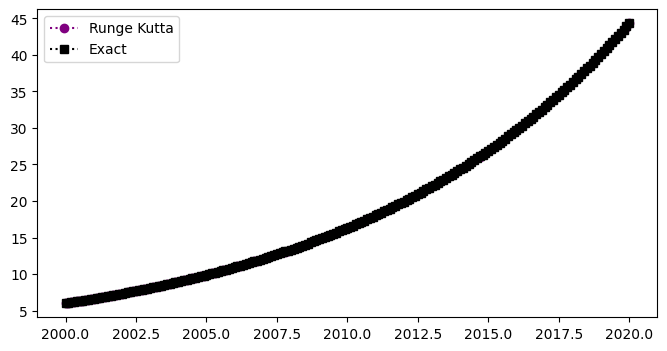
y=6*np.exp(0.1*(t-2000))
fig = plt.figure(figsize=(8,4))
plt.plot(t,w,'o:',color='purple',label='Runge Kutta')
plt.plot(t,y,'s:',color='black',label='Exact')
plt.legend(loc='best')
plt.show()

../_images/fae1289793a2adfde4030d7ca0c149c7c3950910f228db9337396e8a4f902804.png

Table#

The table below shows the time, the Runge Kutta numerical approximation, \(w\), the exact solution, \(y\), and the exact error \(|y(t_i)-w_i|\) for the linear population equation:

d = {'time t_i': t[0:10],    'Runge Kutta':w[0:10],'Exact (y)':y[0:10],'Exact Error':np.abs(np.round(y[0:10]-w[0:10],10))}
df = pd.DataFrame(data=d)
df

	time t_i	Runge Kutta	Exact (y)	Exact Error
0	2000.0	6.000000	6.000000	0.000000
1	2000.1	6.060300	6.060301	0.000001
2	2000.2	6.121206	6.121208	0.000002
3	2000.3	6.182724	6.182727	0.000003
4	2000.4	6.244861	6.244865	0.000004
5	2000.5	6.307621	6.307627	0.000005
6	2000.6	6.371013	6.371019	0.000006
7	2000.7	6.435042	6.435049	0.000007
8	2000.8	6.499714	6.499722	0.000009
9	2000.9	6.565036	6.565046	0.000010

2. Non-Linear Population Equation#

(156)#\[\begin{equation} y^{'}=0.2y-0.01y^2, \ \ (2000 \leq t \leq 2020), \end{equation}\]

with the initial condition,

(157)#\[\begin{equation}y(2000)=6.\end{equation}\]

Specific 2nd Order Runge Kutta for the Non-Linear Population Equation#

To write the specific 2nd Order Runge Kutta method we need

(158)#\[\begin{equation}f(t,y)=0.2y-0.01y^2,\end{equation}\]

this gives

(159)#\[\begin{equation}k_1=f(t_i,w_i)=0.2w_i-0.01w_i^2,\end{equation}\]

(160)#\[\begin{equation}k_2=f(t_i+h,w_i+hk_1)=0.2(w_i+hk_1)-0.01(w_i+hk_1)^2,\end{equation}\]

and the difference equation

(161)#\[\begin{equation}w_{i+1}=w_{i}+\frac{h}{2}(k_1+k_2),\end{equation}\]

for \(i=0,...,199\), where \(w_i\) is the numerical approximation of \(y\) at time \(t_i\), with step size \(h\) and the initial condition

(162)#\[\begin{equation}w_0=6.\end{equation}\]

def nonlinfun(t,w):
    ftw=0.2*w-0.01*w*w
    return ftw

w=np.zeros(N+1)
w[0]=6.0
## 2nd Order Runge Kutta
for k in range (0,N):
    k1=nonlinfun(t[k],w[k])
    k2=nonlinfun(t[k]+h,w[k]+h*k1)
    w[k+1]=w[k]+h/2*(k1+k2)

Results#

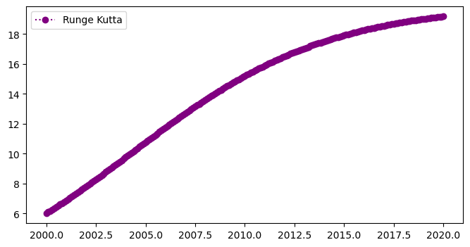
The plot below shows the Runge Kutta numerical approximation, \(w\) (circles) for the non-linear population equation:

fig = plt.figure(figsize=(8,4))
plt.plot(t,w,'o:',color='purple',label='Runge Kutta')
plt.legend(loc='best')
plt.show()

../_images/3c6950ffb085fc68516a808ef5b727ff3fe5bdc4181735af1fb9ca26b14e7e81.png

Table#

The table below shows the time and the Runge Kutta numerical approximation, \(w\), for the non-linear population equation:

d = {'time t_i': t[0:10], 
     'Runge Kutta':w[0:10]}
df = pd.DataFrame(data=d)
df

	time t_i	Runge Kutta
0	2000.0	6.000000
1	2000.1	6.084332
2	2000.2	6.169328
3	2000.3	6.254977
4	2000.4	6.341270
5	2000.5	6.428197
6	2000.6	6.515747
7	2000.7	6.603909
8	2000.8	6.692672
9	2000.9	6.782025

3. Non-Linear Population Equation with an oscilation#

(163)#\[\begin{equation} y^{'}=0.2y-0.01y^2+\sin(2\pi t), \ \ (2000 \leq t \leq 2020), \end{equation}\]

with the initial condition,

(164)#\[\begin{equation}y(2000)=6.\end{equation}\]

Specific 2nd Order Runge Kutta for the Non-Linear Population Equation with an oscilation#

To write the specific 2nd Order Runge Kutta difference equation for the intial value problem we need

(165)#\[\begin{equation}f(t,y)=0.2y-0.01y^2+\sin(2\pi t),\end{equation}\]

which gives

(166)#\[\begin{equation}k_1=f(t_i,w_i)=0.2w_i-0.01w_i^2+\sin(2\pi t_i),\end{equation}\]

(167)#\[\begin{equation}k_2=f(t_i+h,w_i+hk_1)=0.2(w_i+hk_1)-0.01(w_i+hk_1)^2+\sin(2\pi (t_i+h)),\end{equation}\]

and the difference equation

(168)#\[\begin{equation}w_{i+1}=w_{i}+\frac{h}{2}(k_1+k_2),\end{equation}\]

for \(i=0,...,199\), where \(w_i\) is the numerical approximation of \(y\) at time \(t_i\), with step size \(h\) and the initial condition

(169)#\[\begin{equation}w_0=6.\end{equation}\]

def nonlin_oscfun(t,w):
    ftw=0.2*w-0.01*w*w+np.sin(2*np.math.pi*t)
    return ftw

w=np.zeros(N+1)
w[0]=6.0
## 2nd Order Runge Kutta
for k in range (0,N):
    k1=nonlin_oscfun(t[k],w[k])
    k2=nonlin_oscfun(t[k]+h,w[k]+h*k1)
    w[k+1]=w[k]+h/2*(k1+k2)

Results#

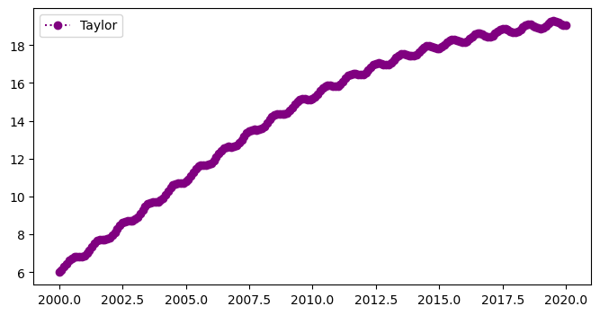
The plot below shows the 2nd order Runge Kutta numerical approximation, \(w\) (circles) for the non-linear population equation:

fig = plt.figure(figsize=(8,4))
plt.plot(t,w,'o:',color='purple',label='Taylor')
plt.legend(loc='best')
plt.show()

../_images/57a3c1f16d3c988c317e6ebd7c9e418e3c71d6149e0f729ab16b0c6d4aea3c6a.png

Table#

The table below shows the time and the 2nd order Runge Kutta numerical approximation, \(w\), for the non-linear population equation:

d = {'time t_i': t[0:10], 
     'Runge Kutta':w[0:10]}
df = pd.DataFrame(data=d)
df

	time t_i	Runge Kutta
0	2000.0	6.000000
1	2000.1	6.113722
2	2000.2	6.276109
3	2000.3	6.458005
4	2000.4	6.623032
5	2000.5	6.741504
6	2000.6	6.801784
7	2000.7	6.814712
8	2000.8	6.809444
9	2000.9	6.822305

Application of 2nd order Runge Kutta to Populations Equations

Contents

Application of 2nd order Runge Kutta to Populations Equations#

2nd Order Runge Kutta#

1. Linear#

2. Non-Linear Population Equation#

3. Non-Linear Population Equation with an oscillation#

Setting up Libraries#

Discrete Interval#

1. Linear Population Equation#

Exact Solution#

Specific 2nd Order Runge Kutta#

Plotting Results#

Table#

2. Non-Linear Population Equation#

Specific 2nd Order Runge Kutta for the Non-Linear Population Equation#

Results#

Table#

3. Non-Linear Population Equation with an oscilation#

Specific 2nd Order Runge Kutta for the Non-Linear Population Equation with an oscilation#

Results#

Table#