Blank Euler Method

The more general form of a first order Ordinary Differential Equation is:

(117)\[\begin{equation} y^{'}=f(t,y). \end{equation}\]

This can be solved analytically by integrating both sides but this is not straight forward for most problems. Numerical methods can be used to approximate the solution at discrete points.

Euler method

The simplest one step numerical method is the Euler Method named after the most prolific of mathematicians Leonhard Euler (15 April 1707 – 18 September 1783) .

The general Euler formula for the first order differential equation

(118)\[\begin{equation} y^{'} = f(t,y), \end{equation}\]

approximates the derivative at time point \(t_i\),

(119)\[\begin{equation} y^{'}(t_i) \approx \frac{w_{i+1}-w_i}{t_{i+1}-t_{i}}, \end{equation}\]

where \(w_i\) is the approximate solution of \(y\) at time \(t_i\).

This substitution changes the differential equation into a difference equation of the form

(120)\[\begin{equation} \frac{w_{i+1}-w_i}{t_{i+1}-t_{i}}=f(t_i,w_i). \end{equation}\]

Assuming uniform stepsize \(t_{i+1}-t_{i}\) is replaced by \(h\), re-arranging the equation gives

(121)\[\begin{equation} w_{i+1}=w_i+hf(t_i,w_i). \end{equation}\]

This can be read as the future \(w_{i+1}\) can be approximated by the present \(w_i\) and the addition of the input to the system \(f(t,y)\) times the time step.

## Library
import numpy as np
import math 
import pandas as pd
%matplotlib inline
import matplotlib.pyplot as plt # side-stepping mpl backend
import matplotlib.gridspec as gridspec # subplots
import warnings

warnings.filterwarnings("ignore")

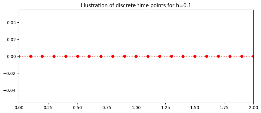
Discrete Interval

The continuous time \(a\leq t \leq b \) is discretised into \(N\) points seperated by a constant stepsize

(122)\[\begin{equation} h=\frac{b-a}{N}. \end{equation}\]

Here the interval is \(0\leq t \leq 2\)

(123)\[\begin{equation} h=\frac{2-0}{20}=0.1, \end{equation}\]

this gives the 21 discrete points:

(124)\[\begin{equation} t_0=0, \ t_1=0.1, \ ... t_{20}=2. \end{equation}\]

This is generalised to

(125)\[\begin{equation} t_i=0+i0.1, \ \ \ i=0,1,...,20. \end{equation}\]

The plot below shows the discrete time steps.

### Setting up time
a=0
b=2.0
N=20


h=(b-a)/(N)
time=np.arange(a,b+h/2,h)
fig = plt.figure(figsize=(10,4))
plt.plot(time,0*time,'o:',color='red')
plt.xlim((a,b))
plt.title('Illustration of discrete time points for h=%s'%(h))
plt.plot();

Initial Condition

To get a specify solution to a first order initial value problem, an initial condition is required.

For our population problem the intial condition is:

(126)\[\begin{equation} y(a)=A. \end{equation}\]

Numerical approximation of Population growth

The differential equation is transformed using the Euler method into a difference equation of the form

(127)\[\begin{equation} w_{i+1}=w_{i}+h f(t_i,w_i). \end{equation}\]

This approximates a series of of values \(w_0, \ w_1, \ ..., w_{N}\).

w=np.zeros(N+1)
w[0]=A ## INITIAL CONDITION
for i in range (0,N):
## ADD EQUATION DYNAMICS TO EQUATION
##    w[i+1]=w[i]+h*

  File "/var/folders/1r/rb8x65yn57q68x042jv2vgx80000gn/T/ipykernel_81484/967930414.py", line 5
    ##    w[i+1]=w[i]+h*
                        ^
SyntaxError: unexpected EOF while parsing