.ipynb .pdf

repository

Contents

Finite Difference Methods for the Poisson Equation

John S Butler john.s.butler@tudublin.ie Course Notes Github

Overview

This notebook will focus on numerically approximating a homogenous second order Poisson Equation.

The Differential Equation

The general two dimensional Poisson Equation is of the form: $$\frac{\partial^2 u}{\partial y^2} + \frac{\partial^2 u}{\partial x^2}=f(x,y), \ \ \ (x,y) \in \Omega=(0,1)\times (0,1),$$with boundary conditions$$U(x,y) = g(x,y), \ \ \ (x,y)\in\delta\Omega\text{ - boundary}.$$

Homogenous Poisson Equation

This notebook will implement a finite difference scheme to approximate the homogenous form of the Poisson Equation $f(x,y)=0$: $$\frac{\partial^2 u}{\partial y^2} + \frac{\partial^2 u}{\partial x^2}=0.$$with the Boundary Conditions:$$u(x,0)=\sin(2\pi x), \ \ \ \ \ 0 \leq x \leq 1, \text{ lower},$$u(x,1)=\sin(2\pi x), \ \ \ \ \ 0 \leq x \leq 1, \text{ upper},$$u(0,y)=2\sin(2\pi y), \ \ \ \ \ 0 \leq y \leq 1, \text{ left},$$u(1,y)=2\sin(2\pi y), \ \ \ \ \ 0 \leq y \leq 1, \text{ right}.$$

# LIBRARY
# vector manipulation
import numpy as np
# math functions
import math 

# THIS IS FOR PLOTTING
%matplotlib inline
import matplotlib.pyplot as plt # side-stepping mpl backend
import warnings
warnings.filterwarnings("ignore")
from IPython.display import HTML
from mpl_toolkits.mplot3d import axes3d
import matplotlib.pyplot as plt

Discete Grid

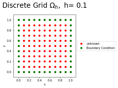
The region $\Omega=(0,1)\times(0,1)$ is discretised into a uniform mesh $\Omega_h$. In the $x$ and $y$ directions into $N$ steps giving a stepsize of $$h=\frac{1-0}{N},$$resulting in$$x[i]=0+ih, \ \ \ i=0,1,...,N,$$and$$x[j]=0+jh, \ \ \ j=0,1,...,N,$$The Figure below shows the discrete grid points for$N=10$, the known boundary conditions (green), and the unknown values (red) of the Poisson Equation.

N=10
h=1/N
x=np.arange(0,1.0001,h)
y=np.arange(0,1.0001,h)
X, Y = np.meshgrid(x, y)
fig = plt.figure()
plt.plot(x[1],y[1],'ro',label='unknown');
plt.plot(X,Y,'ro');
plt.plot(np.ones(N+1),y,'go',label='Boundary Condition');
plt.plot(np.zeros(N+1),y,'go');
plt.plot(x,np.zeros(N+1),'go');
plt.plot(x, np.ones(N+1),'go');
plt.xlim((-0.1,1.1))
plt.ylim((-0.1,1.1))
plt.xlabel('x')
plt.ylabel('y')
plt.gca().set_aspect('equal', adjustable='box')
plt.legend(loc='center left', bbox_to_anchor=(1, 0.5))
plt.title(r'Discrete Grid $\Omega_h,$ h= %s'%(h),fontsize=24,y=1.08)
plt.show();

Boundary Conditions

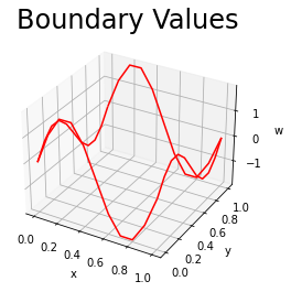
The discrete boundary conditions are $$w_{i0}=w[i,0]=\sin(2\pi x[i]), \text{ for } i=0,...,10, \text{ upper},$$

$$w_{iN}=w[i,N]=\sin(2\pi x[i]), \text{ for } i=0,...,10, \text{ lower},$$

$$w_{0j}=w[0,j]=2\sin(2\pi y[j]), \text{ for } j=0,...,10, \text{ left},$$

$$w_{Nj}=w[N,j]=2\sin(2\pi y[j]), \text{ for } i=0,...,10,\text{ right}.$$

The Figure below plots the boundary values of $w[i,j]$.

w=np.zeros((N+1,N+1))

for i in range (0,N):
        w[i,0]=np.sin(2*np.pi*x[i]) #left Boundary
        w[i,N]=np.sin(2*np.pi*x[i]) #Right Boundary

for j in range (0,N):
        w[0,j]=2*np.sin(2*np.pi*y[j]) #Lower Boundary
        w[N,j]=2*np.sin(2*np.pi*y[j]) #Upper Boundary

        
fig = plt.figure()
ax = fig.add_subplot(111, projection='3d')
# Plot a basic wireframe.
ax.plot_wireframe(X, Y, w,color='r', rstride=10, cstride=10)
ax.set_xlabel('x')
ax.set_ylabel('y')
ax.set_zlabel('w')
plt.title(r'Boundary Values',fontsize=24,y=1.08)
plt.show()

Numerical Method

The Poisson Equation is discretised using $\delta_x^2$ is the central difference approximation of the second derivative in the $x$ direction $$\delta_x^2=\frac{1}{h^2}(w_{i+1j}-2w_{ij}+w_{i-1j}),$$and$\delta_y^2$is the central difference approximation of the second derivative in the$y$direction$$\delta_y^2=\frac{1}{h^2}(w_{ij+1}-2w_{ij}+w_{ij-1}).$$The gives the Poisson Difference Equation,$$-(\delta_x^2w_{ij}+\delta_y^2w_{ij})=f_{ij} \ \ (x_i,y_j) \in \Omega_h,$$w_{ij}=g_{ij} \ \ (x_i,y_j) \in \partial\Omega_h,$$where$w_ij$is the numerical approximation of$U$at$x_i$and$y_j$. Expanding the the Poisson Difference Equation gives the five point method,$$-(w_{i-1j}+w_{ij-1}-4w_{ij}+w_{ij+1}+w_{i+1j})=h^2f_{ij}$$for$i=1,…,N-1$and$j=1,…,N-1$ which can be written

$$\nabla^2_h w_{ij}=f_{ij}.$$

Matrix form

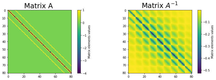
This can be written as a system of $(N-1)\times(N-1)$ equations can be arranged in matrix form $$A\mathbf{w}=\mathbf{r},$$where$A$is an$(N-1)^2\times(N-1)^2$matrix made up of the following block tridiagonal structure$$\left(\begin{array}{ccccccc} T&I&0&0&.&.&.\\ I&T&I&0&0&.&.\\ .&.&.&.&.&.&.\\ .&.&.&0&I&T&I\\ .&.&.&.&0&I&T\\ \end{array}\right),$$where$I$denotes an$N-1 \times N-1$identity matrix and$T$is the tridiagonal matrix of the form:$$T=\left(\begin{array}{ccccccc} -4&1&0&0&.&.&.\\ 1&-4&1&0&0&.&.\\ .&.&.&.&.&.&.\\ .&.&.&0&1&-4&1\\ .&.&.&.&0&1&-4\\ \end{array}\right).$$The plot below shows the matrix$A$and its inverse$A^{-1}$ as a colourplot.

N2=(N-1)*(N-1)
A=np.zeros((N2,N2))
## Diagonal            
for i in range (0,N-1):
    for j in range (0,N-1):           
        A[i+(N-1)*j,i+(N-1)*j]=-4

# LOWER DIAGONAL        
for i in range (1,N-1):
    for j in range (0,N-1):           
        A[i+(N-1)*j,i+(N-1)*j-1]=1   
# UPPPER DIAGONAL        
for i in range (0,N-2):
    for j in range (0,N-1):           
        A[i+(N-1)*j,i+(N-1)*j+1]=1   

# LOWER IDENTITY MATRIX
for i in range (0,N-1):
    for j in range (1,N-1):           
        A[i+(N-1)*j,i+(N-1)*(j-1)]=1        
        
        
# UPPER IDENTITY MATRIX
for i in range (0,N-1):
    for j in range (0,N-2):           
        A[i+(N-1)*j,i+(N-1)*(j+1)]=1
Ainv=np.linalg.inv(A)   
fig = plt.figure(figsize=(12,4));
plt.subplot(121)
plt.imshow(A,interpolation='none');
clb=plt.colorbar();
clb.set_label('Matrix elements values');
plt.title('Matrix A ',fontsize=24)
plt.subplot(122)
plt.imshow(Ainv,interpolation='none');
clb=plt.colorbar();
clb.set_label('Matrix elements values');
plt.title(r'Matrix $A^{-1}$ ',fontsize=24)

fig.tight_layout()
plt.show();

The vector $\mathbf{w}$ is of length $(N-1)\times(N-1)$ which made up of $N-1$ subvectors $\mathbf{w}_j$ of length $N-1$ of the form $$\mathbf{w}_j=\left(\begin{array}{c} w_{1j}\\ w_{2j}\\ .\\ .\\ w_{N-2j}\\ w_{N-1j}\\ \end{array}\right).$$The vector$\mathbf{r}$is of length$(N-1)\times(N-1)$which made up of$N-1$subvectors of the form$\mathbf{r}_j=-h^2\mathbf{f}j-\mathbf{bx}{j}-\mathbf{by}_j$, where$\mathbf{bx}_j $is the vector of left and right boundary conditions$$\mathbf{bx}_j =\left(\begin{array}{c} w_{0j}\\ 0\\ .\\ .\\ 0\\ w_{Nj} \end{array}\right),$$

for $j=1,..,N-1$, where $\mathbf{by}_j$ is the vector of the lower boundary condition for $j=1$,

$$\begin{split} \mathbf{by}_{1} =\left(\begin{array}{c} w_{10}\\ w_{20}\\ .\\ .\\ w_{N-20}\\ w_{N-10}\\ \end{array}\right), \end{split}$$

upper boundary condition for $j=N-1$

$$\begin{split} \mathbf{by}_{N-1} =\left(\begin{array}{c} w_{1N}\\ w_{2N}\\ .\\ .\\ w_{N-2N}\\ w_{N-1N}\\ \end{array}\right), \end{split}$$

for $j=2,...,N-2$ $$\mathbf{by}_j=0,$$and$$\mathbf{f}_j =-\left(\begin{array}{c} 0\\ 0\\ .\\ .\\ 0\\ 0\\ \end{array}\right)$$for$j=1,…,N-1$.

r=np.zeros(N2)

# vector r      
for i in range (0,N-1):
    for j in range (0,N-1):           
        r[i+(N-1)*j]=-h*h*0      
# Boundary        
b_bottom_top=np.zeros(N2)
for i in range (0,N-1):
    b_bottom_top[i]=np.sin(2*np.pi*x[i+1]) #Bottom Boundary
    b_bottom_top[i+(N-1)*(N-2)]=np.sin(2*np.pi*x[i+1])# Top Boundary
      
b_left_right=np.zeros(N2)
for j in range (0,N-1):
    b_left_right[(N-1)*j]=2*np.sin(2*np.pi*y[j+1]) # Left Boundary
    b_left_right[N-2+(N-1)*j]=2*np.sin(2*np.pi*y[j+1])# Right Boundary
    
b=b_left_right+b_bottom_top

Results

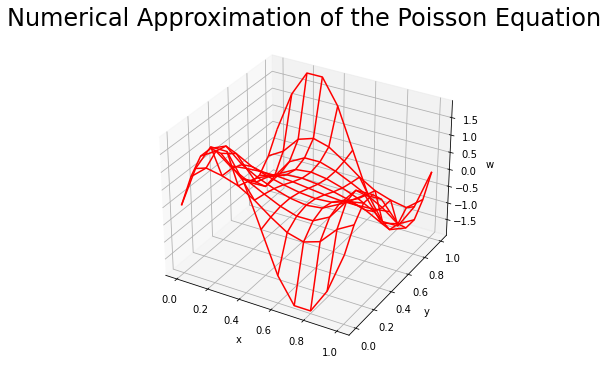
To solve the system for $\mathbf{w}$ invert the matrix $A$ $$A\mathbf{w}=\mathbf{r},$$such that$$\mathbf{w}=A^{-1}\mathbf{r}.$$Lastly, as$\mathbf{w}$ is in vector it has to be reshaped into grid form to plot.

The figure below shows the numerical approximation of the homogeneous Equation.

C=np.dot(Ainv,r-b)
w[1:N,1:N]=C.reshape((N-1,N-1))

fig = plt.figure(figsize=(8,6))
ax = fig.add_subplot(111, projection='3d');
# Plot a basic wireframe.
ax.plot_wireframe(X, Y, w,color='r');
ax.set_xlabel('x');
ax.set_ylabel('y');
ax.set_zlabel('w');
plt.title(r'Numerical Approximation of the Poisson Equation',fontsize=24,y=1.08);
plt.show();

Consistency and Convergence

We now ask how well the grid function determined by the five point scheme approximates the exact solution of the Poisson problem.

Consistency

Consitency (Definition)

Let $$\nabla^2_h(\varphi)=-(\varphi_{i-1j}+\varphi_{ij-1}-4\varphi_{ij}+\varphi_{ij+1}+\varphi_{i+1j})$$denote the finite difference approximation associated with the grid$\Omega_h$having the mesh size$h$, to a partial differential operator$$\nabla^2(\varphi)=\frac{\partial^2 \varphi}{\partial x^2}+\frac{\partial^2 \varphi}{\partial y^2}$$defined on a simply connected, open set$\Omega \subset R^2$. For a given function$\varphi\in C^{\infty}(\Omega)$, the truncation error of$\nabla^2_h$is$$\tau_{h}(\mathbf{x})=(\nabla^2-\nabla^2_h)\varphi(\mathbf{x})$$The approximation$\nabla^2_h$is consistent with$\nabla^2$if$$\lim_{h\rightarrow 0}\tau_h(\mathbf{x})=0,$$for all$\mathbf{x} \in D$and all$\varphi \in C^{\infty}(\Omega)$. The approximation is consistent to order$p$if$\tau_h(\mathbf{x})=O(h^p)$.

In other words a method is consistent with the differential equation it is approximating.

Proof of Consistency

The five-point difference analog $\nabla^2_h$ is consistent to order 2 with $\nabla^2$.

Proof

Pick $\varphi \in C^{\infty}(D)$, and let $(x,y) \in \Omega$ be a point such that $(x\pm h, y),(x,y \pm h) \in \Omega\bigcup \partial\Omega$. By the Taylor Theorem

$$\begin{eqnarray*} \varphi(x\pm h,y)&=&\varphi(x,y) \pm h \frac{\partial \varphi}{\partial x}(x,y)+\frac{h^2}{2!}\frac{\partial^2 \varphi}{\partial x^2}(x,y) \pm\frac{h^3}{3!}\frac{\partial^3 \varphi}{\partial x^3}(x,y)+\frac{h^4}{4!}\frac{\partial^4 \varphi}{\partial x^4}(\zeta^{\pm},y) \end{eqnarray*}$$

where $\zeta^{\pm} \in (x-h,x+h)$. Adding this pair of equation together and rearranging , we get $$\frac{1}{h^2}[\varphi(x+h,y)-2\varphi(x,y)+\varphi(x-h,y) ] -\frac{\partial^2 \varphi}{\partial x^2}(x,y)=\frac{h^2}{4!}\left[\frac{\partial^4 \varphi}{\partial x^4}(\zeta^{+},y)+ \frac{\partial^4 \varphi}{\partial x^4}(\zeta^{-},y) \right]$$By the intermediate value theorem$$\left[\frac{\partial^4 \varphi}{\partial x^4}(\zeta^{+},y)+ \frac{\partial^4 \varphi}{\partial x^4}(\zeta^{-},y) \right] =2\frac{\partial^4 \varphi}{\partial x^4}(\zeta,y),$$for some$\zeta \in (x-h,x+h)$. Therefore,$$\delta_x^2(x,y) =\frac{\partial^2 \varphi}{\partial x^2}(x,y)+\frac{h^2}{2!}\frac{\partial^4 \varphi}{\partial x^4}(\zeta,y)$$Similar reasoning shows that$$\delta_y^2(x,y) =\frac{\partial^2 \varphi}{\partial y^2}(x,y)+\frac{h^2}{2!}\frac{\partial^4 \varphi}{\partial y^4}(x,\eta)$$for some$\eta \in (y-h,y+h)$. We conclude that$\tau_h(x,y)=(\nabla-\nabla_h)\varphi(x,y)=O(h^2).$

Convergence

Definition

Let $\nabla^2_hw(\mathbf{x}_j)=f(\mathbf{x}_j)$ be a finite difference approximation, defined on a grid mesh size $h$, to a PDE $\nabla^2U(\mathbf{x})=f(\mathbf{x})$ on a simply connected set $D \subset R^n$. Assume that $w(x,y)=U(x,y)$ at all points $(x,y)$ on the boundary $\partial\Omega$. The finite difference scheme converges (or is convergent) if $$\max_j|U(\mathbf{x}_j)-w(\mathbf{x}_j)| \rightarrow 0 \mbox{ as } h \rightarrow 0.$$

Theorem (DISCRETE MAXIMUM PRINCIPLE).

If $\nabla^2_hV_{ij}\geq 0$ for all points $(x_i,y_j) \in \Omega_h$, then $$\max_{(x_i,y_j)\in\Omega_h}V_{ij}\leq \max_{(x_i,y_j)\in\partial\Omega_h}V_{ij},$$If$\nabla^2_hV_{ij}\leq 0$for all points$(x_i,y_j) \in \Omega_h$, then$$\min_{(x_i,y_j)\in\Omega_h}V_{ij}\geq \min_{(x_i,y_j)\in\partial\Omega_h}V_{ij}.$$

Propositions

1. The zero grid function for which $U_{ij}=0$ for all $(x_i,y_j) \in \Omega_h \bigcup \partial\Omega_h$ is the only solution to the finite difference problem $$\nabla_h^2U_{ij}=0 \mbox{ for }(x_i,y_j)\in\Omega_h,$$U_{ij}=0 \mbox{ for }(x_i,y_j)\in\partial\Omega_h.$$

2. For prescribed grid functions $f_{ij}$ and $g_{ij}$, there exists a unique solution to the problem $$\nabla_h^2U_{ij}=f_{ij} \mbox{ for }(x_i,y_j)\in\Omega_h,$$U_{ij}=g_{ij} \mbox{ for }(x_i,y_j)\in\partial\Omega_h.$$

Definition

For any grid function $V:\Omega_h\bigcup\partial\Omega_h \rightarrow R$, $$||V||_{\Omega} =\max_{(x_i,y_j)\in\Omega_h}|V_{ij}|,$$||V||_{\partial\Omega} =\max_{(x_i,y_j)\in\partial\Omega_h}|V_{ij}|.$$

Lemma

If the grid function $V:\Omega_h\bigcup\partial\Omega_h\rightarrow R$ satisfies the boundary condition $V_{ij}=0$ for $(x_i,y_j)\in \partial\Omega_h$, then $$||V_||_{\Omega}\leq \frac{1}{8}||\nabla_h^2V||_{\Omega}.$$

Given these Lemmas and Propositions, we can now prove that the solution to the five point scheme $\nabla^2_h$ is convergent to the exact solution of the Poisson Equation $\nabla^2$.

Convergence Theorem

Let $U$ be a solution to the Poisson equation and let $w$ be the grid function that satisfies the discrete analog $$-\nabla_h^2w_{ij}=f_{ij} \ \ \mbox{ for } (x_i,y_j)\in\Omega_h,$$w_{ij}=g_{ij} \ \ \mbox{ for } (x_i,y_j)\in\partial\Omega_h.$$Then there exists a positive constant$K$such that$$||U-w||_{\Omega}\leq KMh^2,$$where$$M=\left\{ \left|\left|\frac{\partial^4 U}{\partial x^4} \right|\right|_{\infty}, \left|\left|\frac{\partial^4 U}{\partial y^4} \right|\right|_{\infty} \right\}$$

Proof

The statement of the theorem assumes that $U\in C^4(\bar{\Omega})$. This assumption holds if $f$ and $g$ are smooth enough. \begin{proof} Following from the proof of the Proposition we have $$(\nabla_h^2-\nabla^2)U_{ij}=\frac{h^2}{12}\left[ \frac{\partial^4 U}{\partial x^4}(\zeta_i,y_j)+\frac{\partial^4 U}{\partial y^4}(x_i,\eta_j) \right],$$for some$\zeta \in (x_{i-1},x_{i+1})$and$\eta_j\in(y_{j-1},y_{j+1})$. Therefore,$$-\nabla_h^2U_{ij}=f_{ij}-\frac{h^2}{12}\left[ \frac{\partial^4 U}{\partial x^4}(\zeta_i,y_j)+\frac{\partial^4 U}{\partial y^4}(x_i,\eta_j) \right].$$If we subtract from this the identity equation$-\nabla_h^2w_{ij}=f_{ij}$and note that$U-w$vanishes on$\partial\Omega_h$, we find that$$\nabla_h^2(U_{ij}-w_{ij})=\frac{h^2}{12}\left[ \frac{\partial^4 U}{\partial x^4}(\zeta_i,y_j)+\frac{\partial^4 U}{\partial y^4}(x_i,\eta_j) \right].$$ It follows that

$$||U-w||_{\Omega}\leq\frac{1}{8}||\nabla_h^2(U-w)||_{\Omega}\leq KMh^2.$$

previous

Numerical Analysis

next

Finite Difference Methods for the Poisson Equation with Zero Boundary